
notes-17-25
Lec 17 (Trees)
Def && Property of trees
两个 equivalent def of trees:
- 无 cycle 的 connected graph
- 一个 graph,其中任意两个 node 之间的 paths 都存在唯一的 shortest one. (这个定义和 1 等价,因为这当且仅当没有 cycle. 如果有 cycle, 那么 cycle 之间一定存在两个点,有多个 path 都是 shortest 的)
Properties:
-
如果一个 tree 有 n 个顶点,那么它一定有 n-1 个 edges. $$ 这个性质是源于:tree 是一个连通图。
by induction.
base case: 单点图;
如果要加入一个顶点,那么必须把它连接到当前的图上。所以必须添加 edge.
但是,由于当前的图是 connected 的,一旦这个新顶点连接了超过一个其他顶点,那么它就会形成 cycle,因为它连接的两个顶点也相互连接了。
所以,tree 中任意一个新加入的顶点都只带来一条边。
并且,这条性质还可以用来 decide tree:
一个有 |V|-1 条边的连通图一定是 tree.
其实这三条性质:边数n-1,连通,无环中只要有两条就可以推导出另一条并表明这是一个树
-
只要往 tree 中加入任意一条新的边,就会形成 cycle
也是 by 连通图的定义
-
只要在 tree 中去掉任意一条边,就会 disconnect
-
每个 tree 都是二分图. (图是二分图当且仅当不包含奇数长度的环
Types: Simple(Undirected) / Rooted(Directed)
Tree 可以被分为 simple tree 和 rooted tree
tree 中,任何 node 都可以作为 root.
-
simple tree 就是不特定选择 root 的 tree,rooted tree 就是选定了一个 node 作为 root 的 tree
可以视作 simple tree 是 undirected 的,rooted tree 是 directed 的。因为 rooted tree 的所有 edges 都可以视作 directed away from the root.
-
Ordered tree 是一种 rooted tree,选定了一个 root 并且给 children of each node 进行 linear ordering
-
Binary tree 就是任意 node 都有最多两个 children 的 ordered tree
-
Complete binary tree 是一个 depth 为 d 的 tree,其中 depth 1, ...., d-1 都是满的,而最后一层 depth d 中间不能有空缺,空缺必须至多集中在右边。
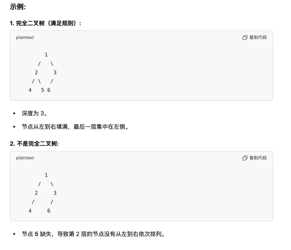
Binary Tree 的 array implementation
- Root 在 index 1(index 0 为 dummy)
- left child of node 在 index
- right child of node 在 index
**binary tree 如果用 arrray 表示,只能以 complete binary tree 的形式进行。**因为我们使用的是连续的内存。当然,tree 本身不一定是 complete 的。在空缺的节点应有标注。
我们发现这个 implementation 的时间复杂度,除了 remove 之外都很好。
- Insert: 平均 O(1),差在结尾。当 tree 当前一层满了要 grow 的时候是 O(n),全部 copy
- Remove: 稍微有些麻烦,不能直接 remove 一个节点不管它的 subtree. 根据需求,要么 fix down 要么删除整个 subtree,但是都要 O(n)
- Parent, child: O(1),直接 n/2, 2n, 2n+1
空间复杂度:tree 越接近 complete 越好,越 sparse 越差。
best case: complete,O(n)
worst case: sparse,每层只有一个,O(2^n)
         1
       /
      2
     /
    4
Binary Tree 的 pointer-based implementation
template <class KEY>
struct Node {
  KEY key,
  Node *left = nullptr;
  Node *right = nullptr;
  Node(const KEY &k)  : key{k} {}
};
优点:首先在空间上优于 array. 总是 O(n)
并且,moving down a tree from parent to child 更加 efficient
Thinking: add parent ?
我们看到 pointer-based implementation 获取 parent 的 complexity 是 O(n) 的. 我们想这完全没必要:为什么不添加一个 parent 变量来直接把它变成 O(1) 呢?
答案是在使用 pointer-based binary tree 作为 data structure 的模型里,我们通常需要 tree 来实现的是它 recursive 的特点,通常不太会需要知道一个 node 的 parent 是什么。
所以功能性地,我们去掉这个变量来减轻 space complexity. 我们获取 parent 的方法是:traverse 整个树.
我们发现这个 implementation 的时间复杂度,除了 remove 之外都很好。
-
Insert: best O(1), worst O(n). binary tree 一般都有需要维持的不变量,比如 BST。insert takes 一个 root 和一个 Key 作为参数,从 root 一层层往下比较进行 insert. 最好的情况 root 是 null, 直接插入;最坏的情况遍历完一整个树。insert 也是一个 recursive 的函数,一层一层 root 下移。
-
Remove: O(n). remove 特别复杂。以 BST 为例。
删除一个节点时分为三种情况:
- 节点是叶子节点:直接删除。
- 节点有一个子节点:用子节点替代被删除的节点。
- 节点有两个子节点:用右子树的最小节点(中序后继)或左子树的最大节点(中序前驱)替代被删除的节点。
-
Parent: O(n),traverse tree
-
child: O(1)
空间复杂度:O(n)
Transfrom a tree into Binary tree
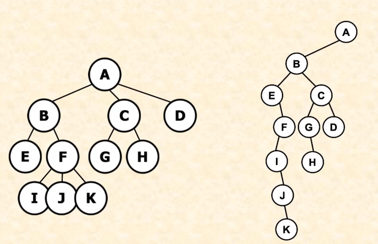
如何 transform 任意一个 tree 为一个 binary tree:
我们使用 left/right children 的关系来取代 sibling 的关系
对于 的所有 children ,我们把 变为 new tree 中 的 left child,而 变为 a chain of right children of
Recursively do this to 的 children . 这样就把所有信息都保存下来了.
Binary Tree Traversal
DFS (Preorder, Inorder, postorder)
preorder:
- visit node
- visit left subtree
- visit right subtree
void preorder(Node *p) {
  if (!p) return;
  visit(p->key);
  preorder(p->left);
  preorder(p->right);
}
inorder
- visit left subtree
- visit node
- visit right subtree
postorder
- visit left subtree
- visit right subtree
- visit node
BFS (levelorder)
Visit nodes in order of increasing depth
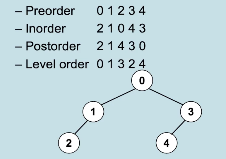
BFS 总是要使用 queue 的. queue 就是一个用来 BFS 的数据结构. 这样总是能保证同一层的被遍历完了开始下一层.
void levelorder(Node *p) {
  if (!p) return;
  queue<Node *>q;
  q.push(p);

  while (!q.empty()) {
    Node *n = q.front();
    q.pop();
    cout << n->key << " ";
    if (n->left) q.push(n->left);
    if (n->right) q.push(n->right);
  }
}
Lec 18 (BST & AVL tree)
BST 是一个 Binary tree, 并满足:
任意一个 node 都比它的 left subtree 中的所有 nodes 要大,比它的 right subtree 中的所有 nodes 要 <=(可以有 duplicate
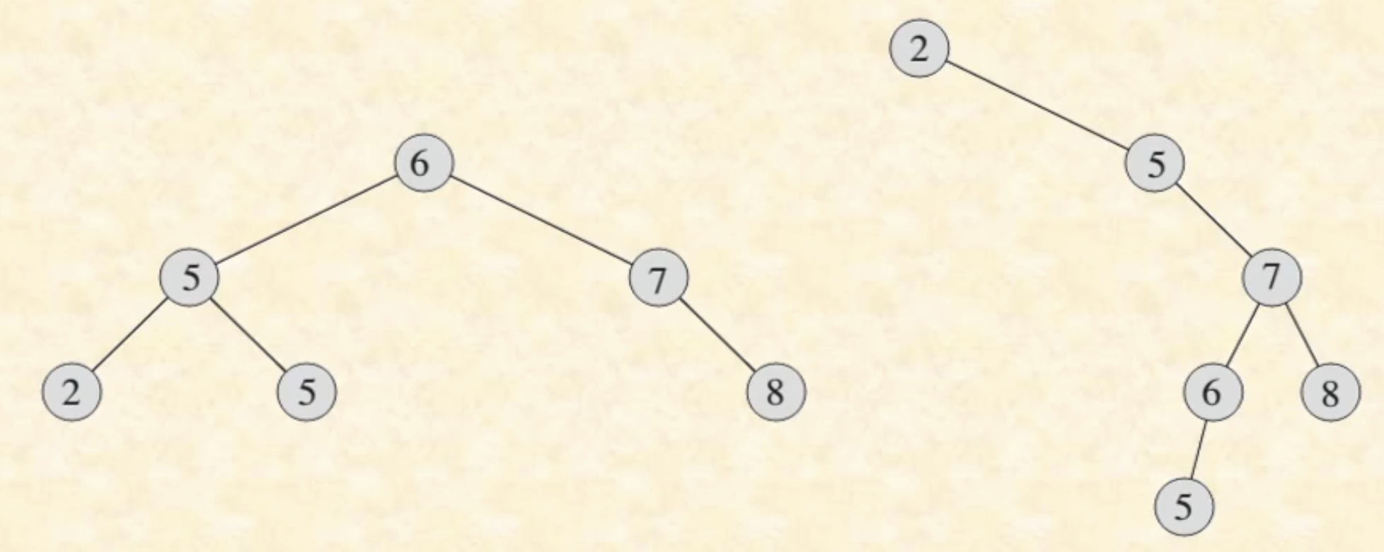
THM:inorder traverse 一个 BST 获得一个 non-decreasing seq.
Which means: 我们可以 do binary search / upper/lower_bound on BST.
并且这个 binary search 由于树的结构,比 array 上的更简单
binary search on BST
Node *tree_search(Node *x, KEY k) {
  while (x != nullptr && k!= x->key) {
    if (k < x-> key) x = x-> left;
    else x = x-> right;
  }
  return x;
}
得到的是一个自顶向下的 path.
O(logn) average.
worst case: 退化成链表的 BST. 一个 stick. 只有这种极端情况有 O(n).
insert in BST
和 search 相似.
找到 upper bound 和 lower bound,在中间插入.
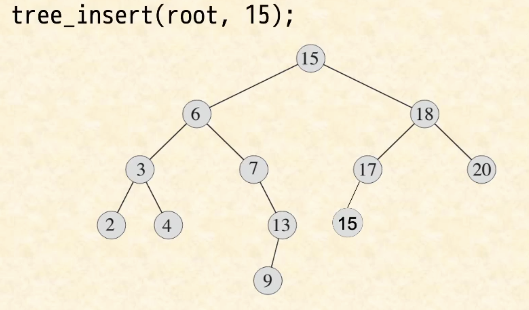
注意:我们需要一个没有唯一答案的 deterministic policy 来处理 duplicate. 放在左边还是右边?取决于我们对
v ? current then search left
v ? current then search right
的处理. STL 使用 <, >=
(也可以使用 <=, >
void BST_insert(Node *&x, KEY k) {
  if (x == nullptr)
    x = new Node(k);
  else if (k < x-> key)
    BST_insert(x->left, k);
  else
    BST_insert(x->right, k);
}
不论是插入还是搜索,处理 binary tree 的核心在于 rebase root,对左子树和右子树分别处理.
Complexity:
对于 well-balanced BST,O(log n)
对于 stick, 退化成链表的 BST,worst case,O(n)
average O(log n)
实际上对于任意一组数据,都存在一个排列方式能触发 worst case(比如 sorted 的)
实际上触发 worst case 居然挺容易的。
这也是为什么我们需要一个可以 self balance 的 binary tree. 等下讲
exercise: find min
找到 leftmost 即可
Node *tree_min(Node *x) {
  if (x == nullptr)
    return nullptr;
 	while (x->left)
    x = x->left;
  return x;
}
Average: O(log n)
Worst: O(n)
remove in BST
Cases:
- no children (trivial)
- no left child
- no right child
- has two children
case 2,3 即:replace the current node by its left/right child. 也是等于 trivial 的.
case 4 有一点难度.
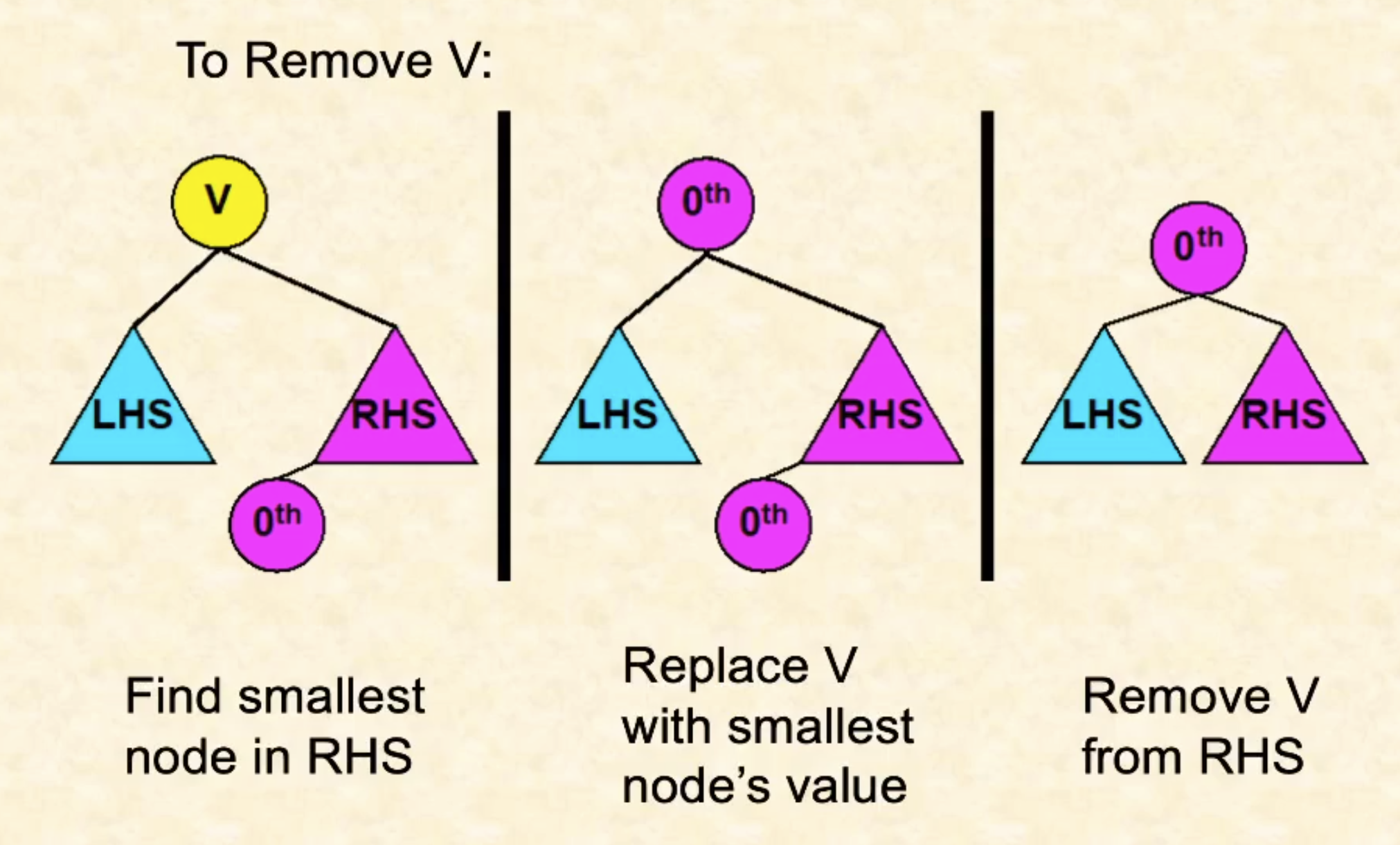
when v has both children
observe: left subtree 中所有的元素,都比 right subtree 要小!
所以:我们把 right subtree 中最小的一个元素(一定是 leaf)拿出来 replace v 就可以了
称这个
template <class T>
void BinaryTree<T>::remove(Node *&tree, const T &val) {
	Node *nodeToDelete = tree;
  Node *inorderSuccessor;

  // first find the position containing the value to remove
  if (!tree) return;
  else if (val < tree->value) remove(tree->left, val);
  else if (val > tree->value) remove(tree->right, val);

  // do remove
  else {
    // two trivial cases
    if (tree->left == nullptr) {
      tree = tree->right;
      delete nodeToDelete;
    }
    if (tree->right == nullptr) {
      tree = tree->left;
  		delete nodeToDelete;
    }
    // real shit
    else {
      inorderSuccessor = tree->right;
      //find the inorderSuccessor
      while (inorderSuccessor->left != nullptr){
        inorderSuccessor = inorderSuccessor->left;
      }
      // replace the value of the node with the value of the succssor
      nodeToDelete->value = inorderSuccessor->value;
      // do one more round, just to remove the original inorderSuccessor
      remove(tree->right, inorderSuccessor->value);
    }
  }
}
仍然是 average O(logn),worst O(n).
AVL tree
BST 不足之处在于 worst case 总是 O(n) 的. 当数据插入的顺序不巧比较 sorted 时,我们会得到一个几乎退化成链表的 BST,使得所有行为都接近 O(n). 我们希望有一个能自动 balance 自己的 BST.
所以就有了 AVL tree. 名字来自发明者
AVL tree 是一种 self-balancing BST. Self-balancing 的意思是 AVL tree 有 Height Balance Property: 对于任意 internal node,它的左右 subtrees 的 height 差别 <=1
这个性质的实现是它依靠 rotation 来 correct imbalance.
Height Balance Property 使得 AVL tree 的 search, insert, remove 达到 worst case O(logn)
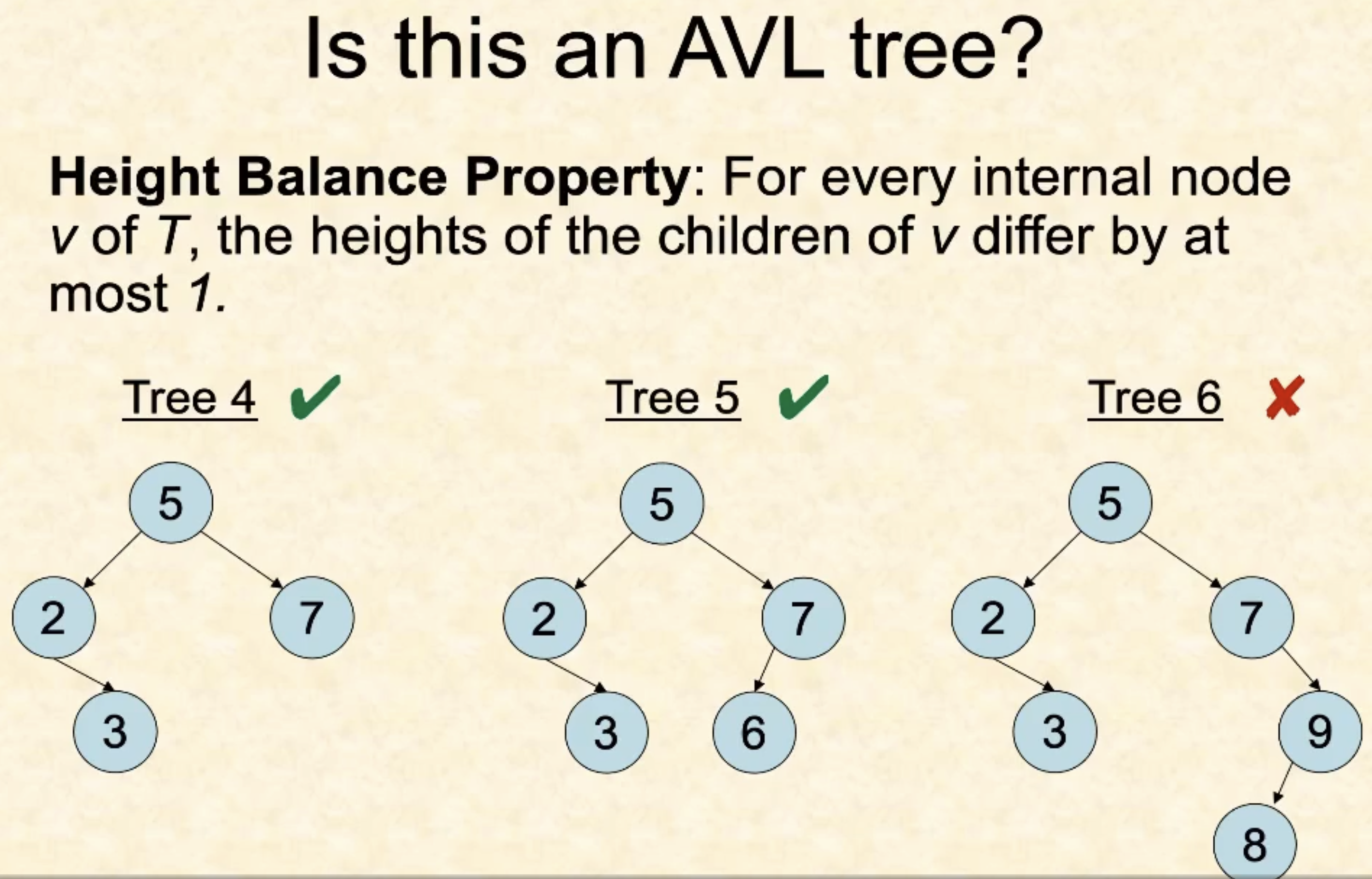
虽然这很显然,但是我们也可以证明它:
不妨考虑 AVL 树的最极端情况:任意左右树 height 都相差了 1
Let 表示 height 的 tree 的 ndoes 数量:
Then $$ for all h >= 2
因而 $$
AVL: insert
AVL tree 的 search 和 sort 就是普通的 BST.
它维持 Height Balance Property 的方法是 insertion 时维持. (以及 remove)
基本 idea: 先正常 insert,然后 rearrange tree to balance height
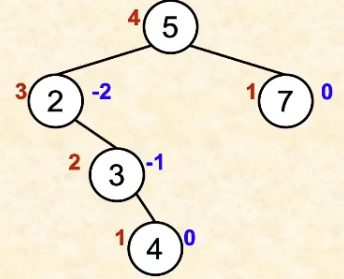
compute balance
AVL tree 中的每个元素都 record 其 height.
计算一个 node 的 balance factor:
balance(n) = height(n->left) - height(n->right)
balance = 0, 1, -1 的都是 AVL-balanced node.
|balance| > 1: out of balance
rotation
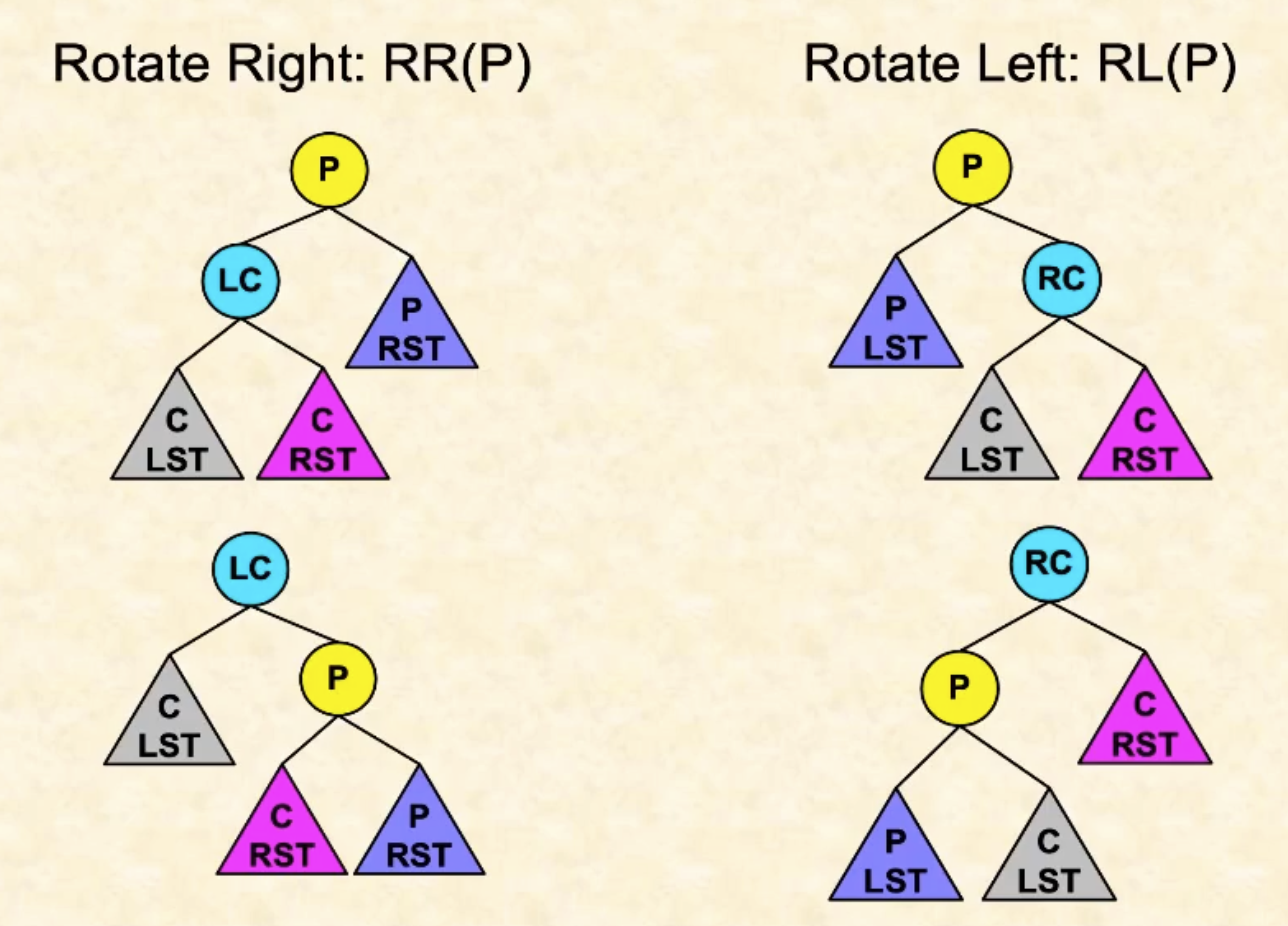
rotation 是一个 local change involving 三个 subtree ptrs 和两个 nodes.
right rotation:
让 left child and left subtree of 提到 root 上, 再把原本的 root 作为它的 right subtree,wtih 原本的 right subtree 成为 的 left subtree
left rotation:
把 right child and right subtree of 提到 root 上,再把原本的 root 作为它的 left subtree,with 原本的 left subtree 成为 的 right subtree
(dually)
容易验证,这保持了 BST 结构.
AVL::Node* AVL::rotate_left(AVL::Node* node) {
    Node *rightchild = node->right;
    Node *rightleftchild = rightchild->left;
    node->right->left = node;
    node->right = rightleftchild;
    fixHeightBelow(rightchild);
    return rightchild;
}

AVL::Node* AVL::rotate_right(AVL::Node* node) {
    Node *leftchild = node->left;
    Node *leftrightchild = leftchild->right;
    node->left->right = node;
    node->left = leftrightchild;
    fixHeightBelow(leftchild);
    return leftchild;
}
how to keep balance in AVL
到底应该以哪个 Node 为 root 来 rotate 左右 subtree 呢?
冷静分析:
AVL tree,在插入一个节点前一定保持平衡,
插入一个节点后,它下面的 subtree 的任意节点 balance factor 一定不变,而它的 siblings 以及它们的 subtree 的任意节点的 balance factor 也一定不变。换言之,balance factor 可能改变以至于不 balance 的只有它到 root 的这段 path 上的节点. 并且显然,balance 的绝对值至多为 2.
一旦检测到 balance 绝对值为 2,设想这个时候,我们找到第一个 unbalance 的节点 :它的 left, right subtree 不平衡,高度差距 =2. ** 这其中蕴含了一个推论,就是它的两个 subtree 中至少有一边一定 >= 两层.**
并且,由于之前所有的 node 的 balance factor 绝对值都 <=1,我们知道这两个 subtree 中长的一边的左右 subtree ( 的subsubtree) 的左右一定从等高变成了不等高,否则之前就不会平衡.
所以,这里一定出现了三个高度:
- 的短子树,最短
- 的长子树的一边子树,其中间
- 的长子树的另一边子树,最长
并且注意到, 的长子树的两边子树高度差距正好为 1,否则在插入前就不平衡;而 的长子树的长子树和 的短子树的高度差距正好为 2,导致了这个 imbalance.
所以只要把这三个树的顺序换一换就好了
Four cases of balance = 2 problem
example:
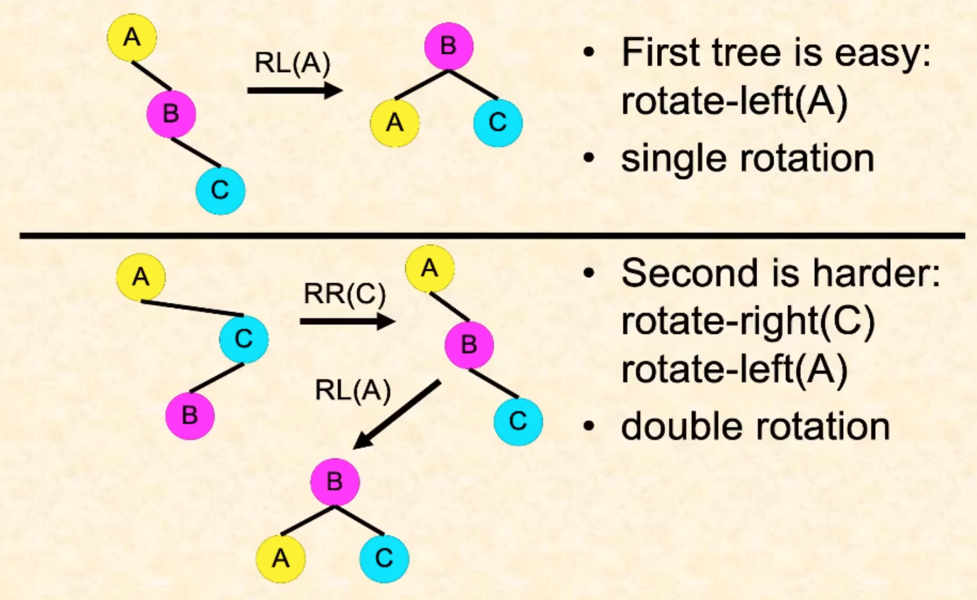
我们发现,一次 rotation 并不能保证解决一切问题. 但是所幸,两次可以解决一切问题。因为一共只有 4 个情况。
我们称为 left left, right right, left right, right left case
LL, RR 最简单. 旋转一次如图.
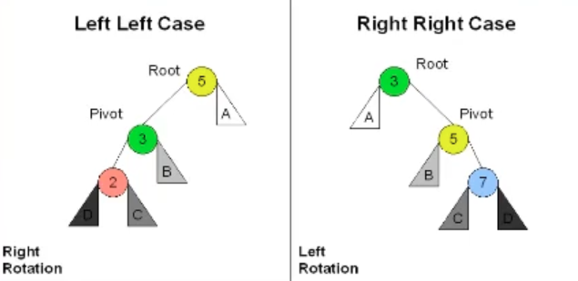
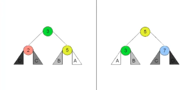
LR, RL 旋转两次. (第一次先转换成 LL, RR.)
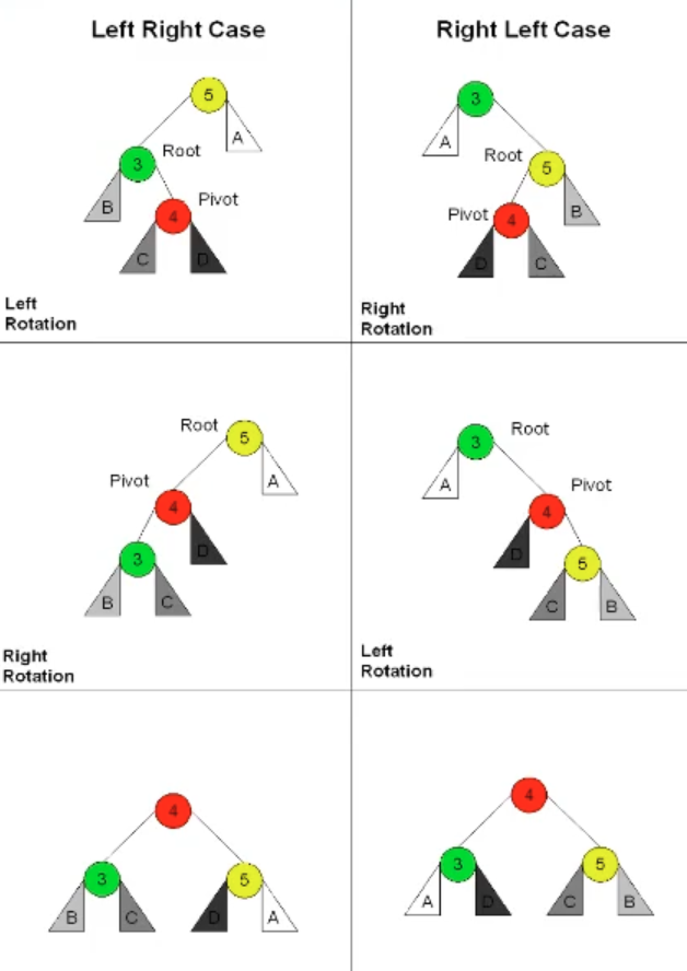
具体的代码:
我们根本不需要在 imbalance 被发现时遍历树来找到第一个 imbalanced node,而是通过 recursion 找到应该插入的点时自动检测 imbalance,而后直接查询是四个情况中的哪一个.
recursion 是自顶向下的,但是 stack 是自底向上一个一个完成的。insert 的复杂度等于 search,因为它等于我们 search 并在每个 stack 都完成一次 fix_height 和可能 rotate. 这两个行为是 O(1) 的.
search 是 O(log n) 的, insert 等于执行 O(log n) 个 O(1) behavior,是 O(log n) 的.
AVL::Node* AVL::insert_node(AVL::Node* node, int datum) {
    if (node == nullptr) {
        // at a leaf position in the tree, so create a new node
        return new Node{ datum, 1, nullptr, nullptr }; // it has height 1
    }

    if (datum < node->datum) {
        node->left = insert_node(node->left, datum);
        node->fix_height(); // remember to fix the height of a node after modifying its children

       // Left Left Case
        if (node->balance()>1 && node->left->balance() >=0) return rotate_right(node);
        // Right Right Case
        if (node->balance()<-1 && node->right->balance()<=0) return rotate_left(node);
        // Left Right Case
        if (node->balance()>1 && node->left->balance()<0) {node->left = rotate_left(node->left);
            return rotate_right(node);}
        // Right Left Case
        if (node->balance()<-1 && node->right->balance()>0) {node->right = rotate_right(node->right); return rotate_left(node);}
    }
    else {
        node->right = insert_node(node->right, datum);
        node->fix_height(); // remember to fix the height of a node after modifying its children

        // Left Left Case
        if (node->balance()>1 && node->left->balance() >=0) return rotate_right(node);
        // Right Right Case
        if (node->balance()<-1 && node->right->balance()<=0) return rotate_left(node);
        // Left Right Case
        if (node->balance()>1 && node->left->balance()<0) {node->left = rotate_left(node->left);
            return rotate_right(node);}
        // Right Left Case
        if (node->balance()<-1 && node->right->balance()>0) {node->right = rotate_right(node->right); return rotate_left(node);}
    }
    return node;
}
Lec 19 (Graphs)
graph. set of a vertices collection and an edges collection.
simple / non-simple ?
(non-simple: 可以有同一个顶点到自己的 edge)
directed / undirected ?
(directed 的表示方式是一条 edge 的第一个第二个顶点表示顺序)
weighted / unweighted ?
(weighted 的表示方式是 edge 加一个组成部分)
Complete / Dense / Sparse graph
Complete graph: 每个节点都和其他所有节点 connect,一共有 |V| * |V-1| / 2 等于 |V|*2 - 2|V| + 1 个 edges
Dense graph 和 sparse graph 不是严格的数学概念。
Dense graph 表示 |E| 和 |V|^2 大小差距较小的 graph. Sparse graph 表示 |E| 和 |V|^2 大小差距较大的 graph (|E| 和 |V| 差不多大).
显然所有 tree 都是 sparse 的,因为 |E| = |V| - 1
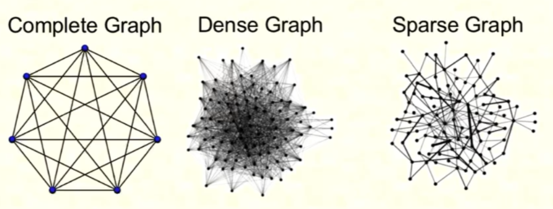
区分 dense graph 和 sparse graph 的目的是:我们通常用 adjacency matrix 来表示 dense graph,用 adjacency list 来表示 sparse graph.
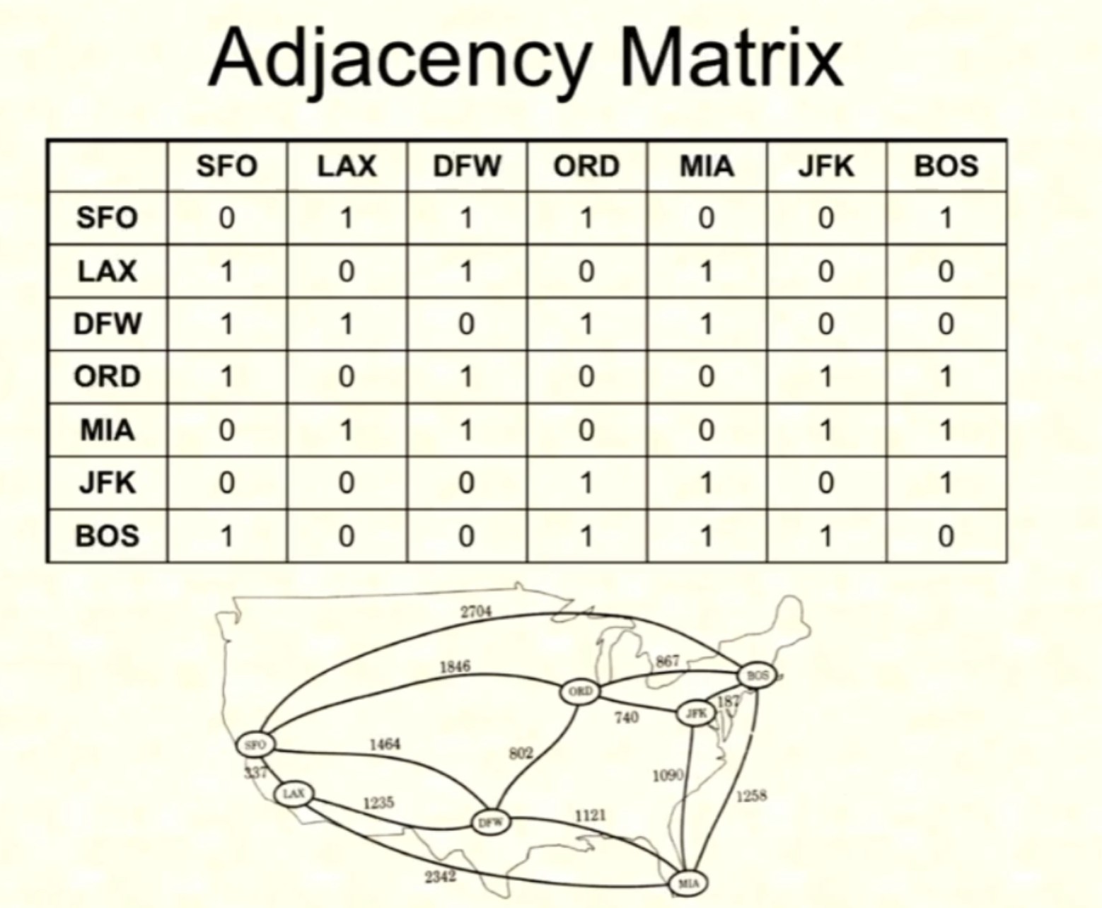
adjacency matrix 展现出的是 |V|^2 个 entry,表示每个点和每个点,包括自己和自己之间(容许non-simple)有没有边;可以接受 directed graph,用横竖来表示方向;可以接受 weighted graph,使用其变体 distance matrix. adjacency matrix 的 cost 也大,如果是一个 sparse graph 的话则大部分 entry 都是 0 (distance matrix 的话是 infty)
Representing a graph: Adjacency matrix
Adjacency matrix 适合用来表示比较 dense 的 graph.(对于 unweighted graph,0 表示无 edge,1表示有 egde;对于 weighted graph,infty 表示无 edge,每个 entry 上表示 edge value)
Space: |V|^2
查看两个顶点是否有边:O(1)
修改和删除边:O(1)
遍历某个顶点的所有 neighbor: O(|V|)
遍历整个图:O(|V|^2)
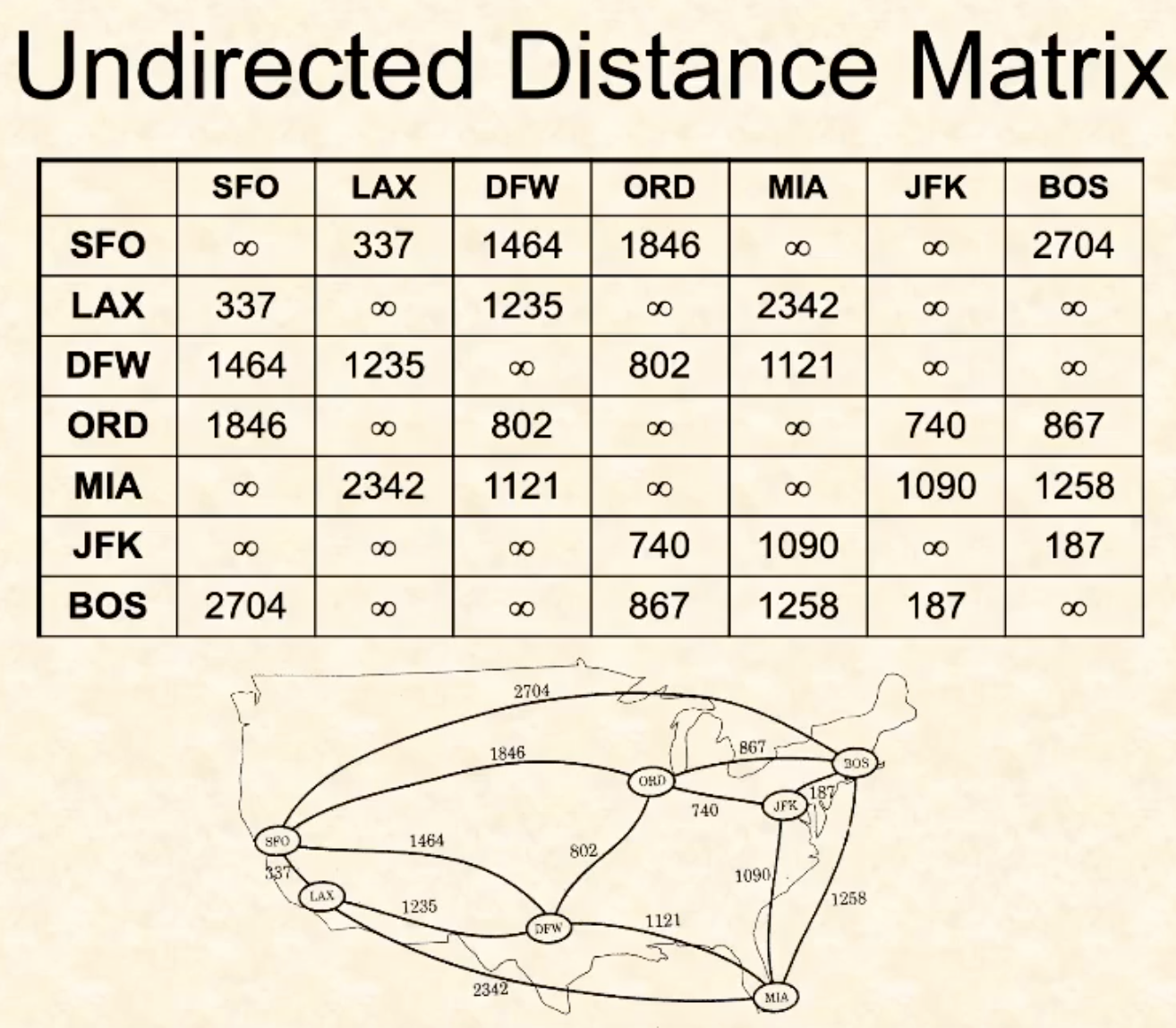
在 C++ 中表示 infty
#include <limits>
double infty = std::numeric_limits<double>::infinity();
它和有限非 0 数的任何操作都得到自己
如果使用 VS 的集成编译系统,那么它除以自己得到 1,乘以 0 得到 0,减去自己得到 0
如果自己使用 g++ 编译,那么这三个行为都得到 nan (not a number).
Representing a graph: Adjacency list
Adjacency list 适合用来表示比较 sparse 的 graph.
它的做法就是建立一个 vector of vectors,第一层数量等于 |V|,每个 vector 都是一个 vertex 的 vertex list
于是:假设 edges 是随机分布的,每个 vertex 的 vertex list 长度是 O(E/V)
space 是: O(1+|E|/|V|) for each vertex,O(|V|+|E|) 总共(这是显然的因为一共的 entries 数量就是 |E|)
找到一个 edge 的 time:O(|E| / |V|)
Adajacency list 表示 directed, weighted graph
用 adjacency list 表示 directed graph:很简单,对于 undirected graph,每条边都会在两个顶点的 vertex list 中各出现一次;而对于 directed graph,每条边只会出现在起点的 vertex list.
表示 unweighted graph:每个 vertex list 是 a list of vertices;表示 weighted graph:每个 vertex list 是 a list of pairs,一个 pair 是一个 vertex 和一个表示 weight 的数.
常见的 Complexity Analysis
-
查看两点间是否有边
Matrix: 全部 O(1),直接 random access
List: worst O(|V|),best O(1),average O(1 + |E| / |V|),即遍历一个 list
-
查找离一个点最近的一个点
Matrix:全部 O(|V|),找一行
List:worst O(|V|),best O(1),average O(1 + |E| / |V|),即遍历一个 list
这些是最基本的操作。而我们在图上还有一些常用操作:比如查找最短路径,这是我们在图上最常用的操作
有三个方法:
- **DFS:只适用于 trees!**在 general 的 graph 上回由于 multiple paths 出现问题
- BFS:只适用于 unweighted graph
- Dijstra:广泛适用于 weighted graph
DFS 找最短路: 只适用于 tree 性质的图
伪代码:
DFS(G):
	mark the root as visited
	push root to stack
	while (stack not empty):
		get and pop top
    for each child of top:
    	if child visited:
    		mark visited
    		push child to top of stack
    		if child is the goal
    			return success
  return failure
DFS 只能找到两个顶点之间的一个 path,但是不保证是什么样的 path
如果这个图是一个 tree,那么就可以用 DFS 找最短路,因为任意两个节点之间一定只有一条路,这条路就是最短路
但是一旦不是 tree,那么找到的 path 就不是最短 path.
方法是把其中一个节点作为 root(recall:tree 中任何节点都可以作为 root!)从它起,深度优先遍历它的所有 subtree,也就是整个 graph
流程:我们放一个 stack,先把作为 root 的起点放进去
while stack 非空:把 top 弹出,top 的所有 neighbor 全部放进 stack
(这样遍历实际上不是一根到底的,而是把 root 所有 children 都放进去,再遍历所有 children 中最右边 children 的所有 chilren,一直遍历到把右节点耗尽,然后从下往上遍历完 root 的最右子树,然后向左传播
time:
- for list: O(1 + |E| / |V|) for each vertex list,因而是 O(|V| + |E|)
- for matrix: O(|V|^2)
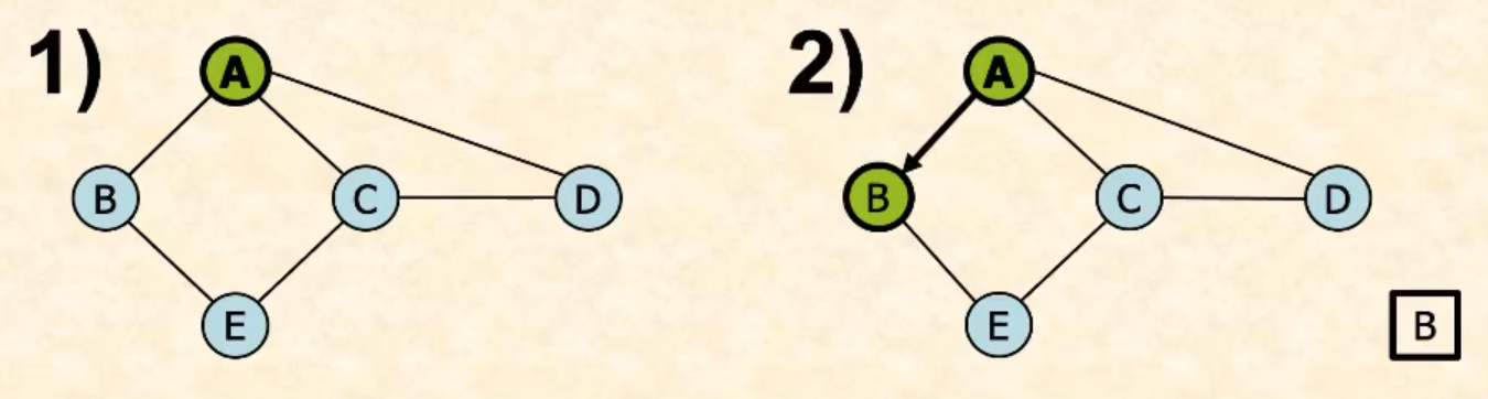
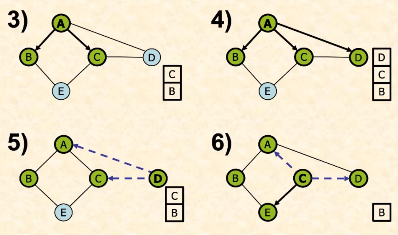
Remember:存一个 parent vector 表示每个 node 的上一个 node 是什么,通过回溯来决定 path 长度
class GraphMatrix {
public:
    std::vector<std::vector<int>> matrix; // 邻接矩阵
    int vertices;                         // 顶点数

    // DFS 只能确保在最短路唯一的情况下找到最短路,其他情况找到的路径不是最短的
    int dfs(int start, int target) {
     	  int path_length = 0;
      	std::vector<int> path;
        std::vector<bool> visited(vertices, false);
        std::stack<int> search;
        std::vector<int> parent(vertices, -1);
        search.push(start);
        visited[start] = true;

        while (!search.empty()) {
            int current = search.top(); search.pop();

            // found: backtrace
            if (current == target) {
                int v = target;
                path_length = 0;
                while (v != -1) {
                    path.push_back(v);
                    int p = parent[v];
                    if (p != -1) {
                        path_length += matrix[p][v];
                    }
                    v = p;
                }
                return path_length;
            }

            for (int i = 0; i < vertices; ++i) {
                if (matrix[current][i] != 0 && !visited[i]) {
                    visited[i] = true;
                    parent[i] = current;
                    search.push(i);
                }
            }
        }
        return -1;
    }
};
BFS 找最短路: 只适用于 unweighted graph
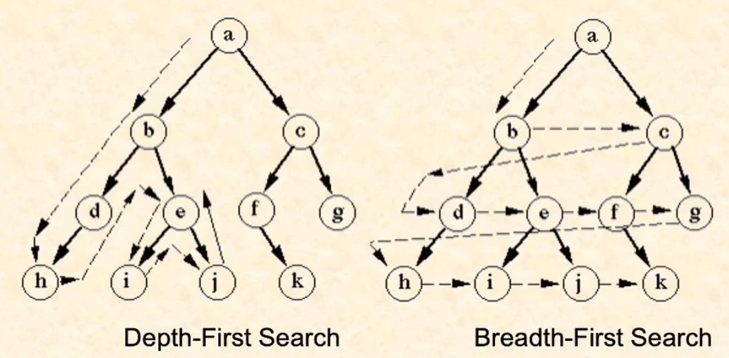
BFS 的流程和 DFS 的流程唯一的差别是用的是 queue 而不是 stack.
BFS 能够在 unweighted graph 上找到最短路的原因就是:以起点为 root,BFS 每遍历一层,离起点的距离就远了一层。所以第一次找到终点,一定是最短的距离
		// BFS 找最短路(仅适用于无权图或等权图)
    int bfs(int start, int end) {
        std::queue<int> q;
        std::vector<bool> visited(vertices, false);
        std::vector<int> distance(vertices, -1);
        std::vector<int> parent(vertices, -1);
        q.push(start);
        visited[start] = true;
        distance[start] = 0;

        while (!q.empty()) {
            int current = q.front();
            q.pop();

            if (current == end) {
                int pathLength = 0;
                int node = end;
                while (node != -1 && node != start) {
                    node = parent[node];
                    pathLength+=1;
                }
                return pathLength;
            }

            for (int i = 0; i < vertices; ++i) {
                if (matrix[current][i] != 0 && !visited[i]) {
                    q.push(i);
                    visited[i] = true;
                    parent[i] = current;
                    distance[i] = distance[current] + 1;
                }
            }
        }
        return -1; // 未找到路径
    }
time: 同 BFS
- for list: O(1 + |E| / |V|) for each vertex list,因而是 O(|V| + |E|)
- for matrix: O(|V|^2)
Dijkstra 找最短路
DFS 和 BFS 找最短路本质上都是:遍历图,把找到的第一条路作为最短路。
而它们的限制其实就是在什么情况下它们找到的第一条路就是最短路:DFS 是在只有一条路的情况下,BFS 是在权重全部相同的情况下。这些都是极端情况。
找 single source 最短路的普遍算法是 Dijstra.
Dijstra 可以找到:对于单个 source,其他所有的 nodes 到这个 source 的最短距离
思路:
-
记一个 distance vector,表示所有 nodes 到 source 的距离
初始化:dist[source] = 0,dist[其他] = infty
-
记一个 visited vector,表示哪些端点还没有被 visit 过(visit 指作为主顶点更新和它所有 neighbors 的 min distance)
一直到所有端点都被 visit 完之前,持续 visit 当前没有被 visit 过的顶点中 dist 最小的一个,称之为 ,访问它的所有 neighbors,尝试更新 的每个 neighbor 的 dist 值:经过 是否能让它的距离变短? $$
这是一个 greedy 的算法。
Dijkstra(G, s)
  for all u ∈ V \ {s}, d(u) = ∞
  d(s) = 0
  R = {}
  while R 6= V
  	pick u not in R with smallest d(u)
  	R = R ∪ {u}
  	for all vertices v adjacent to u
  		if d(v) > d(u) + l(u, v)
  			d(v) = d(u) + l(u, v)
Proof: Invariant Hypothesis of Dijkstra
Claim: 每次循环后,如果不是所有的 unvisited nodes 的 dist 都是无穷,那么 unvisited nodes 中 dist 最短的那个一定是最终形态;
(因而,我们每次都选择当前 dist 最短的 unvisited node 来 visit,最后一定可以得到所有 nodes 和 source 都是最短距离)
Base case: source 距离自己的路径长度是 0.
Inductive step: 假设现在所有 visited 的 nodes 的 dist 已经是最终形态,且当前存在dist 非 infty 的 nodes;WTS:目前 unvisited 的 nodes 中当前 dist 最短的 node 是最终形态
Pf: suppose for contradiction 它不是最终形态
那么之后存在一条路径达到它,这条路径的距离比更新它的时候检查的所有 neighbors 中转达到它更加短
关键事实:这条路径在到达 前,要么全部都是当前的 visited nodes,要么存在当前的 unvisited nodes
case(1)上一个节点是当前的 visited node:由于 visited nodes 的 dist 已经全部 finalize 了,在访问这些 nodes 的过程中已经把它们的 neighbors,包括 在内,更新到了当前 visited nodes 能够涵盖的最小。既然这条路所有的 nodes 都 visited 过了,那么这个 path 的长度就是当前的 dist(u). 所以矛盾
case(2)路径上存在至少一个 unvisited node:令 为这条路径上第一个 unvisited node.
注意:决定选择 作为准备 visit 的 node 的时候,也查看了 !由于我们选择了 ,这个时候从 visit 过的确认是最短路径的任何节点,到其他 unvisited 节点,到 要比到 更远!
那么由于每个 edge 长度都是非负的,从 到 的这段路径非负,
已知最终的 dist(u) = 当前的 dist(v) + v到u的某段路径,而当前的 dist(v) 又比当前的 dist(u) 大,当前的 dist(u) 比最终的 dist(u) 大。矛盾
下面就是上述的 Dijkstra 的 implementation
Naive Dijkstra
const int INF = INT_MAX;
// 不使用优先队列的 Dijkstra 算法
void dijkstraWithoutPQ(int n, int source, vector<vector<pair<int, int>>> &graph) {
    vector<int> dist(n, INF);       // 最短距离数组
    vector<bool> visited(n, false); // 是否访问过

    dist[source] = 0;
    for (int i = 0; i < n; ++i) {
        int u = -1;
        int minDist = INF;
        // 找到未访问节点中距离最小的节点
        for (int j = 0; j < n; ++j) {
            if (!visited[j] && dist[j] < minDist) {
                u = j;
                minDist = dist[j];
            }
        }
        if (u == -1) break; // 所有节点都访问过或者无法到达
        visited[u] = true;

        // 更新相邻节点的距离
        for (auto &edge : graph[u]) {
            int v = edge.first, weight = edge.second;
            if (!visited[v] && dist[u] + weight < dist[v]) {
                dist[v] = dist[u] + weight;
            }
        }
    }
    // 输出结果
    for (int i = 0; i < n; ++i) {
        cout << "Distance from source to node " << i << ": ";
        if (dist[i] == INF) cout << "INF" << endl;
        else cout << dist[i] << endl;
    }
}
复杂度显然是:O(|V|^2 + |E|)
|E| 是更新节点距离的总共消耗,|V|^2 则是遍历所有 vertices list
Dijkstra with PQ
由于我们每次都要选取非 infty 的 unvisited 中最短的一个来作为 visited,我们不如建立一个 PQ.
这样只需要 O(log|V|) 就可以找到最短的
注意到:实际上我们并不需要一个 visited vector 来追踪哪些访问过了哪些没有。使用 PQ 的情况下,我们持续地把新的待开发 neighbors 的 node 放入其中,只要 PQ 还没空就一直按照我们的期望跑下去。如果 PQ 空了,那就说明所有联通 source 的节点都找到了最短路。如果还有节点没有找到,要么它不联通 source,否则一定会在某个 visited node 的轮次内找到更短的路径,从而被放进 PQ。这是我们证明过的。
因而这个版本的 Dijkstra 非常简洁。
// 使用优先队列的 Dijkstra 算法
void dijkstraWithPQ(int n, int source, vector<vector<pair<int, int>>> &graph) {
    vector<int> dist(n, INF); // 最短距离数组
    priority_queue<pair<int, int>, vector<pair<int, int>>, greater<>> pq;

    dist[source] = 0;
    pq.push({0, source}); // {距离, 节点}

    while (!pq.empty()) {
        auto [curDist, u] = pq.top(); pq.pop();
        if (curDist > dist[u]) continue; // 当前路径不优,不处理
        // 更新相邻节点的距离
        for (auto &edge : graph[u]) {
            int v = edge.first, weight = edge.second;
            if (dist[u] + weight < dist[v]) {
                dist[v] = dist[u] + weight;
                pq.push({dist[v], v});
            }
        }
    }

    // 输出结果
    for (int i = 0; i < n; ++i) {
        cout << "Distance from source to node " << i << ": ";
        if (dist[i] == INF) cout << "INF" << endl;
        else cout << dist[i] << endl;
    }
}
Backtracking Dijkstra finding path
这是一个带 backtracking 的 Dijkstra,通过添加一个 prev vector 来追踪具体路径
// 使用优先队列的 Dijkstra 算法,带回溯功能
void dijkstraWithPath(int n, int source, vector<vector<pair<int, int>>> &graph) {
    vector<int> dist(n, INF);          // 最短距离数组
    vector<int> prev(n, -1);           // 前驱节点数组,用于回溯路径
    priority_queue<pair<int, int>, vector<pair<int, int>>, greater<>> pq;

    dist[source] = 0;
    pq.push({0, source}); // {距离, 节点}

    while (!pq.empty()) {
        auto [curDist, u] = pq.top(); pq.pop();

        if (curDist > dist[u]) continue; // 当前路径不优,不处理

        // 更新相邻节点的距离
        for (auto &edge : graph[u]) {
            int v = edge.first, weight = edge.second;
            if (dist[u] + weight < dist[v]) {
                dist[v] = dist[u] + weight;
                prev[v] = u; // 记录前驱节点
                pq.push({dist[v], v});
            }
        }
    }

    // 输出结果:最短距离和路径
    for (int i = 0; i < n; ++i) {
        cout << "Distance from source to node " << i << ": ";
        if (dist[i] == INF) {
            cout << "INF" << endl;
            continue;
        }
        cout << dist[i] << endl;

        // 回溯路径
        cout << "Path: ";
        vector<int> path;
        for (int at = i; at != -1; at = prev[at]) {
            path.push_back(at);
        }
        reverse(path.begin(), path.end()); // 路径需要反转
        for (size_t j = 0; j < path.size(); ++j) {
            cout << path[j];
            if (j < path.size() - 1) cout << " -> ";
        }
        cout << endl;
    }
}
测试:
int main() {
    int n = 5;
    vector<vector<pair<int, int>>> graph(n);
    graph[0].push_back({1, 10});
    graph[0].push_back({4, 5});
    graph[1].push_back({2, 1});
    graph[1].push_back({4, 2});
    graph[2].push_back({3, 4});
    graph[3].push_back({0, 7});
    graph[3].push_back({2, 6});
    graph[4].push_back({1, 3});
    graph[4].push_back({2, 9});
    graph[4].push_back({3, 2});

  	std::cout << "Dijkstra without priority queue:" << std::endl;
    dijkstraWithoutPQ(n, 0, graph);
    std::cout << std::endl;
    std::cout << "Dijkstra with priority queue:" << std::endl;
    dijkstraWithPQ(n, 0, graph);
    std::cout << std::endl;
    std::cout << "Dijkstra with priority queue and path:" << std::endl;
    dijkstraWithPath(n, 0, graph);
}
Lec 20 (MST)
一个 weighted undirected connected graph 的一个 spanning tree 就是它的一个 subgraph,其 connect 所有点并且无 cycle(即是一个 tree)
minimal spaning tree 就是它的所有 spanning tree 中总 weights 和最小的 (可以有多个
Cut Property
Cut Property: 任意地切分一个图(把顶点分为两个集合,其 disjoint union 是整个 V),在 cross 两个顶点集的所有边上,如果其中一条严格小于其他所有边,那么这条边一roof: 个切分,并取它的 crossing edges 中的最短一边。
假设存在一个 MST,称为 T,不包含这条边 e:
由于 T 是 connected 的,这些边中至少有一条,称为 e' ,在 T 中
by 连通图的性质,这两个顶点集组成的两个子图都是连通图,所以去掉 e' 加入 e 后仍然是连通的
于是有 $$ 和 T 是 MST 矛盾了
Corollary: shortest edge for one vertex must be in all MST; in some if unstrict
对于任意一个 edge,我们都可以把它和其他所有顶点分为两个 subgraph(单点集和其他所有点的子图)
所以 by cut property,任意一个顶点 associated 的所有 edges 中如果存在严格最短的,那么这条 edge 一定在所有 MST 中
类似逻辑可证明:任意一个顶点 associated 的所有 edges 中如果存在多个最短的,那么它们都各自在某个 MST 中.
(And Another Trivial Collary: Cycle Property
于图中的任意 cycle,如果其中的一条边比 cycle 中的其他边都严格长,那么它一定不在任何 MST 中。This is trivially true.)
Prim's Algorithm: Using Cut Property
记录三个 vector,每个都 of |V| size
- visited vector:每个 node v 是否被 visited
- minimal edge weight vector: 每个 node v 的 minimal edge weight
- parent vector: 每个 node v 的 parent
Correctness 分析
流程:
-
设置所有的 visited 是 false(not visited);设置 minimal edge weight vector 全部是 infty;设置 parent vector 全部是 -1(no parent)
我们用 k_v 来把整个图分割成两个集合,于是就可以运用 cut property(Corollary: shortest edge for one vertex must be in all MST; in some if unstrict)
minimal weight edges vector 用来保存所有 nodes 在作为 outie set 元素的时候,与 intie set 元素形成的边中最短的一个;于是,遍历整个 outie set,所有的 minimal weight edges 中最短的一个就是 outie set 和 intie set 边缘上最短的边!
-
loop |V| 次,每次选择 intie set 和 outie set 边缘上最短的一个 edge,把它连接的 outie node 加入 intie set 中,这样就无 cycle 地添加了 |V-1| 条 edges,根据连通图的性质,最后一定会得到一个 spanning tree!
每一次我们把一个 node 加入 intie set,我们就更新它所有 neighbors 的边的长度,放入 minimal weight edges vector
这样,我们就总是能 keep track of intie 和 outie 边缘处的边,因为一旦一个 node 变成 intie,它和它周围的 outies 的边就立刻被更新
通过 corollary of cut property,我们可以证明每次携带一条边加入新 node 后,生成的都是某个 MST 的一个 subtree,于是 by 联通图的性质,最后生成的一定是一个完整的 MST!
不使用 heap 的朴素 prim
void primMST(vector<vector<pair<int, int>>> &graph, int V) {
    vector<int> key(V, INT_MAX);   // To store the minimum weight for each vertex
    vector<bool> inMST(V, false);   // To check if a vertex is included in the MST
    vector<int> parent(V, -1);      // To store the parent of each vertex in the MST

    key[0] = 0;   // Start from vertex 0
    for (int count = 0; count < V - 1; count++) {
        int minKey = INT_MAX, u;

        // Find the minimum key vertex not included in the MST
        for (int v = 0; v < V; v++) {
            if (!inMST[v] && key[v] < minKey) {
                minKey = key[v];
                u = v;
            }
        }

        inMST[u] = true; // Include the vertex in the MST

        // Update key value and parent for adjacent vertices
        for (auto &edge : graph[u]) {
            int v = edge.first;
            int weight = edge.second;
            if (!inMST[v] && weight < key[v]) {
                key[v] = weight;
                parent[v] = u;
            }
        }
    }

    // Print the MST
    cout << "Prim's MST:\n";
    for (int i = 1; i < V; i++) {
        cout << parent[i] << " - " << i << "\n";
    }
}
过一个流程:
-
更新第一个 node 进入 intie.
更新它三个 neighbors 的 minimal edges
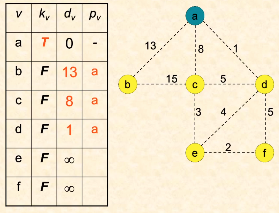
-
进入下一循环,遍历 outie 发现这个时候 intie, outie 的cut 上最短边来自 d
于是把 d 放进 intie,更新 d 周围的 minimal edges.
有四条,其中一条是和 a 的,发现 a 在 intie 里(True),于是这条不更新;其余三条,d 造成的新边都要比老边短,于是更新
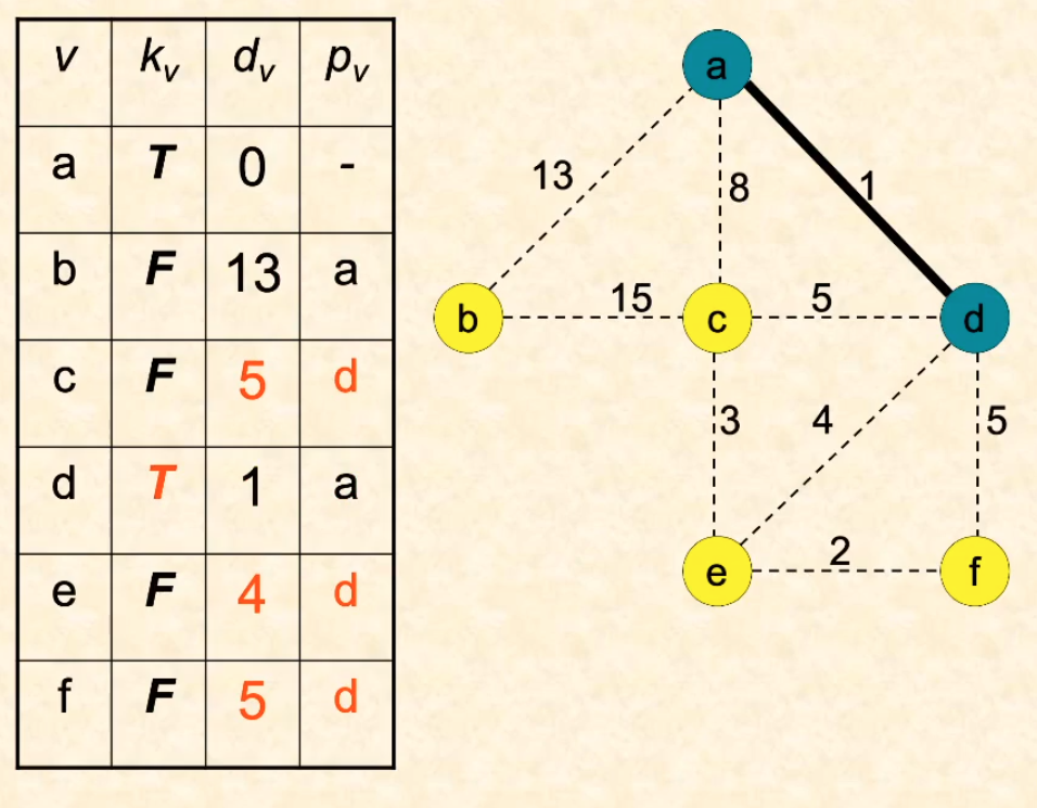
-
下一循环,发现 outies 里最短边来自 e
更新
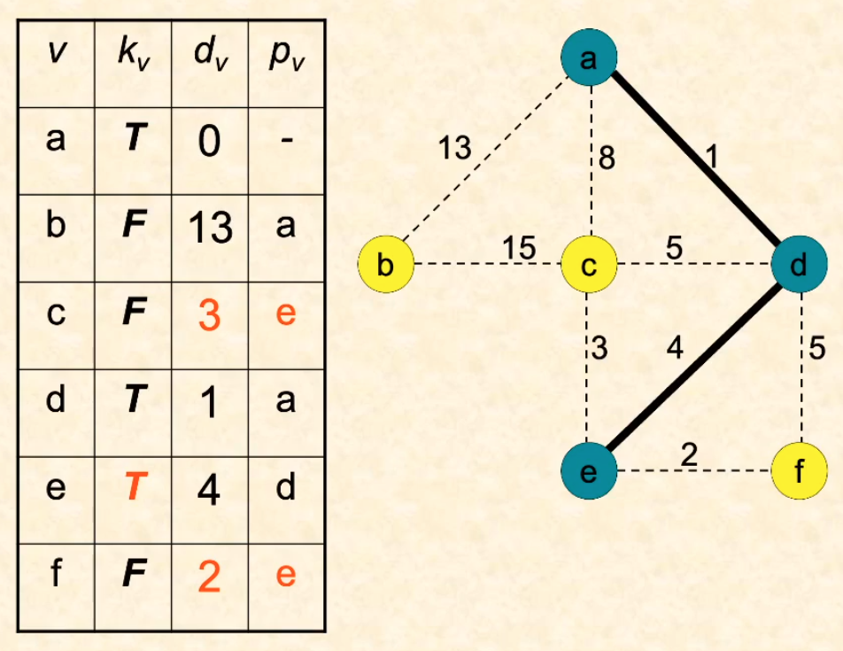
-
更新,下一个最低来自 f
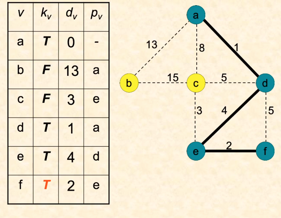
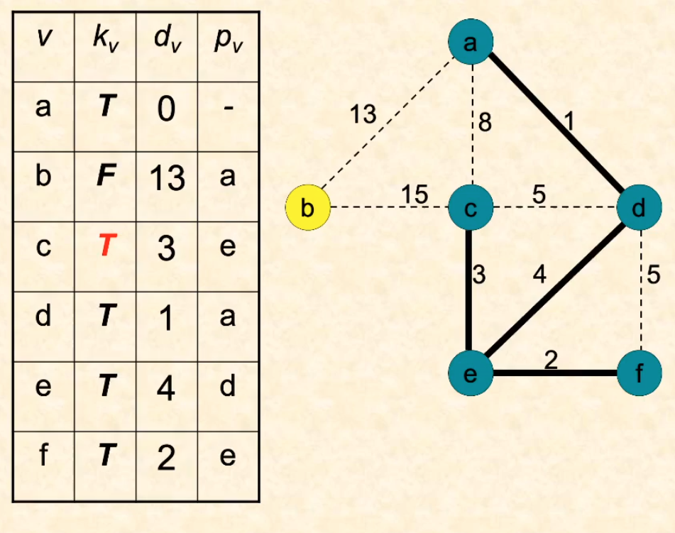
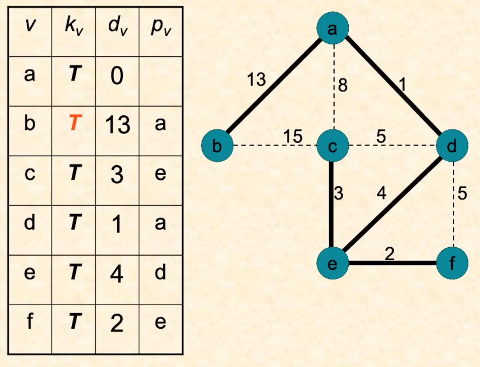
这是一个贪心算法,核心在于每次更新 indie,indie 里所有的 nodes 的三个值都不用再变了,是局部最优。
使用 heap 的 Prim
和 Dijkstra 一样,我们既然每次都要找到 outies 的 minimal edges 里面的最小值,不如起一个 PQ,总能提高运行效率
PQ:每次更新 minimal edges,我们都把更新好的 <node, min_edge_val> 放进 PQ.
这个 implementation 比 Dijkstra 更简单,因为我们处理丢进 PQ 但中途被放进 intie 的 nodes 的方法也很简单:每次从 PQ 中弹出 top 元素,检查它是不是 outie 元素,是的话就正常操作,不是就忽略。
void primMSTHeap(vector<vector<pair<int, int>>> &graph, int V) {
    priority_queue<pair<int, int>, vector<pair<int, int>>, greater<pair<int, int>>> pq;
    vector<int> key(V, INT_MAX);
    vector<bool> inMST(V, false);
    vector<int> parent(V, -1);
    key[0] = 0;

    pq.push({0, 0});  // (weight, vertex)
    while (!pq.empty()) {
        int u = pq.top().second;
        pq.pop();

        if (inMST[u]) continue;	// ignore if already intie
        inMST[u] = true; // Include the vertex in the MST

        // Update key value and parent for adjacent vertices
        for (auto &edge : graph[u]) {
            int v = edge.first;
            int weight = edge.second;
            if (!inMST[v] && weight < key[v]) {
                key[v] = weight;
                parent[v] = u;
                pq.push({key[v], v});
            }
        }
    }

    // Print the MST
    cout << "Prim's MST using Heap:\n";
    for (int i = 1; i < V; i++) {
        cout << parent[i] << " - " << i << "\n";
    }
}
Complexity 分析
-
不使用 heap 的朴素实现
loop: |V|
每个 loop 内,loop 一层 outie 来选择 minimal edge:|V|;更新 neighbors 的 min edges: O(1 + |E|/|V|)
因而是
-
使用 heap 的实现:
While pq nonempty:loop 是 O(|E|) 的
PQ.Getmin: O(log |E|)
在 loop 内遍历更新 neighbors 的 min edges:O(1 + |E|/|V|);
对于每个 neighbor 都 insert PQ: O(log|E|)
因而是
所以使用 heap 未必更快。可以明确的是:在 graph 比较 sparse 的情况下,使用 heap 更快
Minimum-cost egde property
如果 graph 中 minimum cost 的 edge 是 Unique 的,那么它一定在任何 MST 中
proof: 假设存在一个 MST 没有这一边,那么把它放进 T 中 形成一个循环,去掉任意一个其他边仍然是一个 tree
Corollary: sorting property
对一个 connected graph 的所有边长进行排序,前 k 个不形成 cycle 的 edges 一定是某个 MST 的 subgraph。
(因而,前 |V| -1 个不形成 cycle 的 edges 一定一个 MST.)
proof:
Proof by induction.
Base case: k = 0.
Inductive step: 假设 是某个 MST 的 subgraph,并且 e_k 是接下来的最小且和 不形成 cycle
那么我们看向 :把 加入到 中形成了一个 cycle,于是把其中一个边去掉又是一个 tree. 由于有其他边长都大于等于 ,那么一定可以用 来替换这个边
实际上我们可以这么想:
一个 spanning tree 是由一个点作为起点,每加入一条边就是新加入一个顶点。加入 次就结束了
因而当我们固定起点,其实每个新加入的顶点都 associate 了它被加入时的边。
MST 就是让加入每个顶点时它 associate 的边尽量最短
我们选择一个加入后不形成 cycle 的边,其实就是加入一个新的顶点。
我们把所有边都排序好,选择前 个最短的不形成 cycle 的边,就是加入 个其他顶点,并且确保它们的 weights 总和达到最小. 任何其他选择都只不过是换一换两个点加入的顺序和它们加入时 associate 的边,但是这个选择一定不会比我们通过排序获得的选择更好。
Kruskal's Algorithm: Using sorting property
Kruskal's algorithm 就是 sorting property 的直接 application.
算法:我们 sort edges,然后 loop through all edges,跳过形成 cycle 的. Idea 十分简单
如何检测是否有 cycle: union-find set
sorting 很简单,而检测有无 cycle 则需要思考
Idea:当我们想添加一条边的时候,它会形成一个 cycle 当且仅当它的两个顶点已经 connected
所以:我们用一个 union-find set 来 keep track of connectivity.
用两个顶点属于同一个集合来表示 connected,每当放一个新的 edge 等待判断的时候,我们首先查看它们是否在同一个集合
进入 MST 的时候,我们就把它们的顶点 union. (设置其中一个的 parent 为另一个)
note:每次加入新边,一定是带着一个新元素。当所有元素都进入同一个 set,也就意味着 MST 形成。
对于所有不在 MST 中的 nodes,它们的 representative 一定是自己,因为没有修改过。
所以一条边的两个顶点都在 MST subgraph 中,当且仅当它会导致 cycle,当且仅当它的两个顶点被 find 出来发现 root 相同.
这证明了 union-find set 来检测 cycle 的正确性。
// Union-Find Disjoint Set data structure
struct DisjointSet {
    vector<int> parent, rank;
    DisjointSet(int n) : parent(n), rank(n, 0) {
        for (int i = 0; i < n; i++) {
            parent[i] = i;
        }
    }

    int find(int u) {
        if (u != parent[u]) {
            parent[u] = find(parent[u]);
        }
        return parent[u];
    }

    void unite(int u, int v) {
        int rootU = find(u);
        int rootV = find(v);
        if (rootU != rootV) {
            if (rank[rootU] < rank[rootV]) {
                parent[rootU] = rootV;
            } else if (rank[rootU] > rank[rootV]) {
                parent[rootV] = rootU;
            } else {
                parent[rootV] = rootU;
                rank[rootU]++;
            }
        }
    }
};


void kruskalMST(vector<Edge> &edges, int V) {
    sort(edges.begin(), edges.end(), compareEdges);

    DisjointSet ds(V);
    vector<Edge> mst;

    for (auto &edge : edges) {
        if (ds.find(edge.src) != ds.find(edge.dest)) {
            mst.push_back(edge);
            ds.unite(edge.src, edge.dest);
        }
    }

    // Print the MST
    cout << "Kruskal's MST:\n";
    for (auto &edge : mst) {
        cout << edge.src << " - " << edge.dest << "\n";
    }
}
Lab 09 (Graphs)
algorithm problem: decide graph has a cycle
Given: 一个 connected graph with adjacent list
idea: DFS the graph.
每次到一个 Node, mark it as visited.
每次 DFS 的时候,我们有:
- 当前 node 的上一个 node (当前 node 是哪个 node DFS 来的)
- 当前 node
- 当前 node 的 adjacent nodes, 等待 DFS
我们传入当前 node 的上一个 node 为 parent;检查每个新到的 node 是不是当前 node 的 parent 或者 unvisited:如果既不是 parent 又已经 visited 了,那么说明它是一个 back route. 于是一定存在 cycle.
// complexity: O(V + E)
bool is_graph_cyclic(const vector<vector<int>> &adj_list) {
    unordered_set<int> visited;

    // Since the graph is connected, we only need to start from one node (e.g., node 0 or 1)
    return hasCycleDFS(0, -1, adj_list, visited);
}

bool hasCycleDFS(int node, int parent,
                const vector<vector<int>>& adjList,
                unordered_set<int>& visited) {
    visited.insert(node);

    for (int neighbor : adjList[size_t(node)]) {
        // If the neighbor is not visited, recurse
        if (visited.find(neighbor) == visited.end()) {
            return hasCycleDFS(neighbor, node, adjList, visited);
        }
        // If the neighbor is visited and not the parent, we found a cycle
        else {
          if (neighbor != parent)
            return true;
        }
    }
    // reach here: all neighbors are visited, and not parent, then ends
    return false;
}


int main() {
    // Example: Input graph
    const vector<vector<int>> adjList = {
        {2, 3}, //0
        {2},  //1
        {0, 1}, //2
        {0} //3
    };

    if (is_graph_cyclic(adjList)) {
        cout << "Graph contains a cycle" << endl;
    } else {
        cout << "Graph does not contain a cycle" << endl;
    }
Lec 21 (Algorithm Family)
Brute-Force && Greedy Algorithm
简称暴力搜索。
例子:Counting Change
我现在有 1, 2, 5, 10 元的硬币一些,请使用最少的硬币,来 sum up to 元
Brute-Force Algorithm:
对于 个 coins,有 中可能的 subset
把它们全部都列出来,并检查每一种是否 add up to ,keep 当前最少的硬币数量
Complexity:
Def: Greedy Algorithm 就是做出一系列 locally optimal decisions 以取得一个 globally optimal solution(我们不对 locally optimal decisions 做出任何修改);当且仅当我们可以证明 locally optimal decisions lead to globally optimal solution 时,greedy algorithm 是有效的。
Possible Greedy way to Count change:
我们希望 minimize #amounts of coins,to reach sum =
我们发现,把所有 coins 从大到小排列,如果大的 fit in 就直接拿一枚大的硬币 ,再考虑如何 reach
Complexity:
但是这个 greedy 并不成立。
反例:现在有 25,10,1 元硬币,要凑齐 30 元
如果拿了 25 元:那么不得不拿 5 个一元,结果一共拿了 6 个硬币
最优解:3个10元
Lec 22 (Backtracking && branch and bound)
我们介绍两种问题:
-
Constraint Satisfaction Problems:给定很多 Constraints,我们是否能 satisfy 它们所有?如何 satisfy?
可能有多个答案。
ex: sorting
-
Optimization problems:在 satisfy 所有 constraints 的前提下,我们如何 minimize 一个 objective function?
对于 constraint satisfaction problems,backtracking 通常是好的算法;对于 Optimization problems,branch and bound 通常是好的算法
Backtracking: idea
实际上 backtracking 和暴力搜索很像,不同的点在于:我们沿着一个 tree 来 preorder traverse 它,每当发现解行不通时,我们就把当前 node 下面的整个 subtree 给剪掉(称为剪枝),然后回溯到它的 parent node,换一个 child node 继续遍历。
好的剪枝策略可以大大降低时间损耗。
backtracking 的 idea 就是:在庞大的解空间中,通过剪枝来不断削减其大小,最后只需要遍历一小部分 promising 的解,就可以找到所有可能的解
流程
form 1:
Algorithm checknode(node v)
	if (promising(v))
		if (isSol(v))
			done
		else
			for each node u adjacent to v
				checknode(u)
form 2:
Algorithm checknode(node v)
	if (isSol(v))
		good, add to solution set
	else
		for each node u adjacent to v
			if (promising(u))
				checknode(u)
n-queens: 经典 backtracking problem
n-queens 的规则(constraints):
- 同行只能有一个 queen
- 同列只能有一个 queen
- 两个 queen 不能在对角线上
否则就会相互攻击。我们在 n*n 的棋盘上放 n 个 queens,看看有多少种放置方法可以使它们都无法相互攻击。
Idea:
void NQueens::solve() {
    putQueen(0);
}

// promising if would not violate any constraints
bool NQueens::promising(uint32_t row, uint32_t col) {
    return   column[col] == AVAILABLE
        && leftDiagonal[row + col] == AVAILABLE
        && rightDiagonal[row - col + (size - 1)] == AVAILABLE;
}  // NQueens::promising()

// Place a queen in row
// If display == true, display each board as a solution is found
void NQueens::putQueen(uint32_t row) {
    // 如果这个时候已经 proceed 到了最后行, 说明这是一个 sol.
    if (row == size) {++solutions;return;}

    // Check every column within this row
    for (size_t col = 0; col < size; ++col) {
        // Check if proposed placement is promising
        if (promising(row, col)) {
            // Make the move, and a recursive call to next move
            positionInRow[row] = col;
            column[col] = !AVAILABLE;
            leftDiagonal[row + col] = !AVAILABLE;
            rightDiagonal[row - col + (size - 1)] = !AVAILABLE;
            putQueen(row + 1);

            // Undo this move and thus backtrack
            column[col] = AVAILABLE;
            leftDiagonal[row + col] = AVAILABLE;
            rightDiagonal[row - col + (size - 1)] = AVAILABLE;
        }  // if
        ++tried;
    }  // for
}  // NQueens::putQueen()
复杂度:
还是很大,但是比暴力搜索的 要好;并且由于剪枝的建立,实际情况会比 要好。
Branch and Bound: Backtracking with optimization
Solve TSP with Branch and Bound
TSP 问题:给定 n 个城市及它们之间的距离矩阵 dist,找到一条从城市 0 开始,访问所有城市最后回到城市 0 (hamilton cycle)的最短路径。
const int INF = numeric_limits<int>::max();
struct Node {
    int level;       // 当前深度
    int cost;        // 当前路径的代价
    int bound;       // 当前节点的下界
    vector<int> path; // 当前路径
    // PQ 比较函数,小的优先
    bool operator<(const Node& other) const {
        return bound > other.bound;
    }
};

// 计算给定矩阵的最小边界
int calculateBound(const vector<vector<int>>& dist, const vector<int>& path, int n) {
    int bound = 0;

    // 标记已经访问的城市
    vector<bool> visited(n, false);
    for (int city : path) visited[city] = true;

    // 加上路径中已有的代价
    for (size_t i = 1; i < path.size(); ++i) {
        bound += dist[path[i - 1]][path[i]];
    }

    // 为未访问的城市估计下界
    for (int i = 0; i < n; ++i) {
        if (!visited[i]) {
            int minCost = INF;
            for (int j = 0; j < n; ++j) {
                if (i != j && !visited[j]) {
                    minCost = min(minCost, dist[i][j]);
                }
            }
            if (minCost != INF) bound += minCost;
        }
    }

    return bound;
}

// TSP 分支限界主函数
int tspBranchAndBound(const vector<vector<int>>& dist) {
    int n = dist.size();
    priority_queue<Node> pq; // 优先队列,按节点的下界排序
    int bestCost = INF;      // 当前最优解
    vector<int> bestPath;    // 最优路径

    // 初始节点
    Node root;
    root.level = 0;
    root.cost = 0;
    root.path = {0}; // 从城市 0 开始
    root.bound = calculateBound(dist, root.path, n);
    pq.push(root);

    // 分支限界搜索
    while (!pq.empty()) {
        Node curr = pq.top();
        pq.pop();

        // 如果当前节点的下界大于最优解,剪枝
        if (curr.bound >= bestCost) continue;

        // 如果当前路径包含所有城市并回到起点
        if (curr.level == n - 1) {
            // 计算完整路径的代价
            int totalCost = curr.cost + dist[curr.path.back()][0];
            if (totalCost < bestCost) {
                bestCost = totalCost;
                bestPath = curr.path;
                bestPath.push_back(0); // 回到起点
            }
            continue;
        }

        // 生成子节点
        for (int i = 0; i < n; ++i) {
            if (find(curr.path.begin(), curr.path.end(), i) == curr.path.end()) {
                Node child;
                child.level = curr.level + 1;
                child.path = curr.path;
                child.path.push_back(i);
                child.cost = curr.cost + dist[curr.path.back()][i];
                child.bound = child.cost + calculateBound(dist, child.path, n);

                // 如果下界小于当前最优解,加入优先队列
                if (child.bound < bestCost) {
                    pq.push(child);
                }
            }
        }
    }

    // 输出最优路径
    cout << "最优路径: ";
    for (int city : bestPath) {
        cout << city << " ";
    }
    cout << endl;

    return bestCost;
}


int main() {
    // 示例:距离矩阵
    vector<vector<int>> dist = {
        {0, 10, 15, 20},
        {10, 0, 35, 25},
        {15, 35, 0, 30},
        {20, 25, 30, 0}
    };

    int result2 = tspBranchAndBound(dist);
    cout << "Shortest path by branch and bound: " << result2 << endl;

    return 0;
}
Approximation Algorithms
nearest neighbor + 2opt 优化
-
nearest neighbor: 从 node 0 开始,每次都选择最近的未访问 neighbor
这是一个很直白的算法.
O(n^2)
问题在于:在刚开始的时候, 总权重很小,不亚于正确的 TSP 路径;但是越到后面,已访问的nodes多了,就会出现 nodes 比较近的 neighbors 都已经被访问,只能绕远路的情况。因而比较极端的数据会导致误差很大
-
2opt: 对于 nearest neighbor 选取好的路径,尝试选取任意两条不相邻的边 AB, CD 看看能否换成 AC, BD,如果能的话,换了之后能否降低总路径。
while (局部优化无法再提高, 即上一次循环中没有被提高) {
for (all nodes)
for(all other nodes)
...
// if swap succeed, then 局部优化又一次提高了
}
O(n^3)
insertion
分为 nearest, furtherest 以及 arbitratary insertion. 但其实都一样,就是每次加入一个点进入当前的 partial tour,
这个点的选取,根据三个策略有不同,但没有明显的优劣之分
这个点的插入就是在 partial tour 中减去一条边 AB,添加两条边 AC, BC. 我们选择它插入 partial tour 的位置使得 这个 AC+BC-BC 最小,也就是它造成的 distance 的增加最小
-
首先锁定第一个 node 0 和与它最近/最远/随机的 node i,0 to i to 0 形成一个 partial tour
-
每次迭代都是一个 partial tour (subTSP cycle),
(1) for nearest/furtherest: 随便选一个 partial tour 中的 node 里,看看不在 partial tour 中的 nodes 哪个和它最近/最远,选取这个 node 为下一个访问的点;for arbitrary: 随机选取一个不在 partial tour 中的 node 作为下一个访问的点.
(2) 遍历 partial tour,找到插入位置
Lec 23 (DP)
通常的 recursive algorithm 是把整个问题 recursively 划分为 independent 的子问题
而 DP 则用来处理可以分成 subproblems,但它们之间却不 independent 的问题
并且,DP 可以 reduce 一个 recursive function 的 runtime(通过一个 table 储存子问题的 solution,把时间从 O(c^n) exponential 降到 O(n^c) polynomial),是一个用 memory 来 trade time 的做法,这种 technique 叫做 memoization
Memoization
Rewrite 一个 recursive function: On Exit:
Save inputs and the result
On entry:
Check the inputs: whether have seen before
if so, then retrieve the result from memo
Fibo: naive and DP
uint64_t naiveFibo(uint32_t i) {
    if (i == 1 || i == 0) return i;
    return naiveFibo(i-1) + naiveFibo(i-2);
}
O(1.6^n),exponential
uint64_t topDownFibo(uint32_t n) {
    static uint64_t memo[MAX_FIB + 1] = {0, 1}; //initial value
    // if n is too large, not in range of service
    if (n > MAX_FIB) return 0;
    // if already computed, return the value
    if (memo[n] > 0 || n==0) return memo[n];

    memo[n] = topDownFibo(n-1) + topDownFibo(n-2);
    return memo[n];
}
O(n),因为每个 entry 至多只会被计算一次
uint64_t bottomUpFibo(uint32_t n) {
    static uint64_t memo[MAX_FIB + 1] = {0, 1}; //initial value
    for (uint32_t i = 2; i <= n; i++) {
        memo[i] = memo[i-1] + memo[i-2];
    }
    return memo[n];
}
更明显的 O(n)
Binomial Coefficent DP
按照数学公式直接计算:good idea,complexity 也只有 O(n),
但是:仅仅 21! 就能 overflow 一个 int64.
阶乘数实在太大了。所以更加好的办法是使用递归公式: $$ (n 个东西里面选 k 个,就等于
Case 1:第 n 个东西被选中,所以还要在 n-1 个东西里选 k-1 个;
Case 2:第 n 个东西没被选中,所以还要在 n-1 个东西里选 k 个
的情况的相加)
Base case: $$
Recursion 做法:
uint64_t binomialCoeffRecursion(uint32_t n, uint32_t k) {
    if (k == 0 || k == n) return 1;
    return binomialCoeffRecursion(n-1, k-1) + binomialCoeffRecursion(n-1, k);
}
exponential.
Top-Down DP:
uint64_t binomialCoeffHelper(uint32_t n, uint32_t k, vector<vector<uint64_t>>& memo) {
    if (k == 0 || k == n) {
        memo[k][n] = 1;
        return 1;
    }
    if (memo[k][n] > 0) return memo[k][n];
    memo[k][n] = binomialCoeffHelper(n-1, k-1, memo) + binomialCoeffHelper(n-1, k, memo);
    return memo[k][n];
}

uint64_t binomialCoeffTopDown(uint32_t n, uint32_t k) {
    vector<vector<uint64_t>> memo(k+1, vector<uint64_t>(n+1, 0));
    return binomialCoeffHelper(n, k, memo);
}
Bottom-Up DP:
uint64_t binomialCoeffBottomUp(uint32_t n, uint32_t k) {
    vector<vector<uint64_t>> memo(k+1, vector<uint64_t>(n+1));
    for (size_t i = 0; i <= k; i++) {
        for (size_t j = i; j <= n; j++) {
            if (i==j || i==0) memo[i][j] = 1;
            else memo[i][j] = memo[i-1][j-1] + memo[i][j-1];
        }
    }
    return memo[k][n];
}
O(nk)
THM: 任何 top-down DP 都可以转化为 bottom-up DP!
但是,bottom-up 不见得总比 top-down 要轻松
Knight Moves DP
knight 也就是象棋里的马,可以往任何方向直走两格之后再转90度走一格。
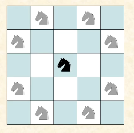
问题:从某个格子 (startX, startY) 出发,走 exactly K 步,有多少种走法可以到另一个格子 (destX, destY)?
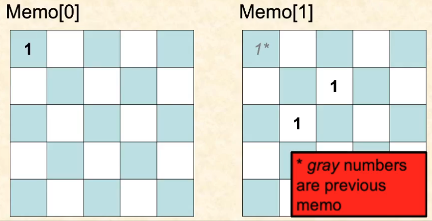
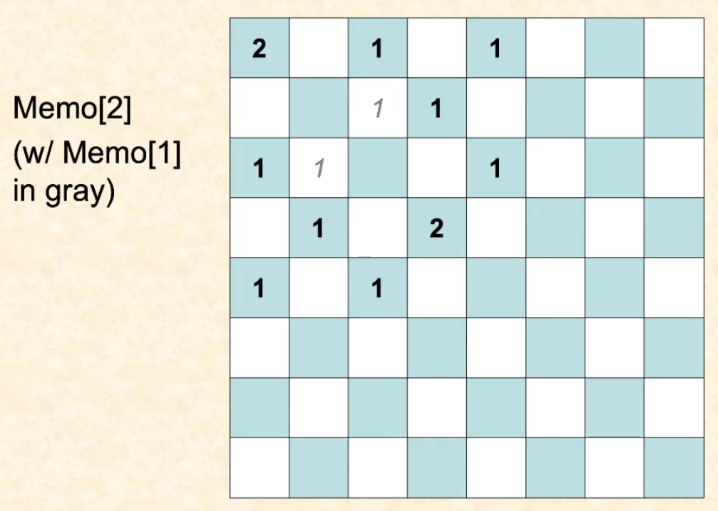
Idea: DP!建立一个 3D table,其中第一个维度表示第几步,第二第三维度是整个棋盘
这是一个简单的 DP. 第 N 步的棋盘就是:遍历第 N-1 步的棋盘,所有 >0 (说明第 N-1 步possible 到达这个地方) 的格子的 possible moves. $$ dp[k][x][y]= \sum_{\text{(nx, ny) 是有效位置}}
dp[k−1][nx][ny]
$$
注意 1:第 N-1 步的棋盘上的一格上面的数字多大,say it is M,就表示 前 N-1 步有 M 种方法在第 N-1 步时到达这个格子,于是第 N-1 步到第 N 步,这个格子上 8 个方向上的 moves 都有 M 重.(直观)也就是 for all 8 directions,dp[k][nx][ny] += dp[k - 1][x][y];
注意 2:超过棋盘边界不算。
int knightMoveDP(int plateWidth, int totalMoves, int startX, int startY, int destX, int destY) {
    // Initialize a 3D DP table with all zeros
    vector<vector<vector<int>>> dp(totalMoves + 1, vector<vector<int>>(plateWidth, vector<int>(plateWidth, 0)));

    // Base case: starting position
    dp[0][startX][startY] = 1;

    // Fill DP table
    for (int k = 1; k <= totalMoves; ++k) {
        for (int x = 0; x < plateWidth; ++x) {
            for (int y = 0; y < plateWidth; ++y) {
                if (dp[k - 1][x][y] > 0) { // If there are paths to this cell
                    for (auto move : knightMoves) {
                        int nx = x + move.first;
                        int ny = y + move.second;
                        if (nx >= 0 && nx < plateWidth && ny >= 0 && ny < plateWidth) { // Valid move
                            dp[k][nx][ny] += dp[k - 1][x][y];
                        }
                    }
                }
            }
        }
    }

    // Print the entire chessboard for the K-th step
    cout << "Chessboard at step " << totalMoves << ":" << endl;
    for (int x = 0; x < plateWidth; ++x) {
        for (int y = 0; y < plateWidth; ++y) {
            cout << dp[totalMoves][x][y] << " ";
        }
        cout << endl;
    }

    // Return the number of paths to (tx, ty) after K moves
    return dp[totalMoves][destX][destY];
}


/*
Chessboard at step 4:
16 0 17 0 18 0 7 0
0 10 0 22 0 8 0 7
17 0 16 0 23 0 10 0
0 22 0 36 0 14 0 9
18 0 23 0 18 0 9 0
0 8 0 14 0 6 0 4
7 0 10 0 9 0 6 0
0 7 0 9 0 4 0 0
*/
时间:
实际运行:每走一步,所有数字的总和大概乘以 8,实际上比 8 小,因为有很多超过边界的。
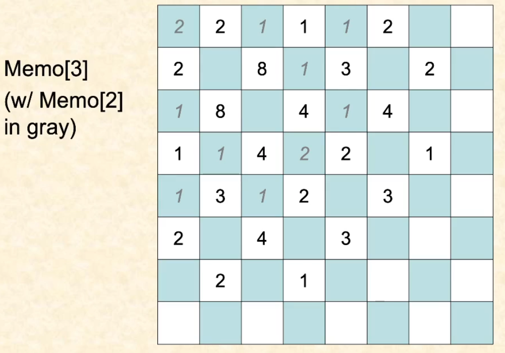
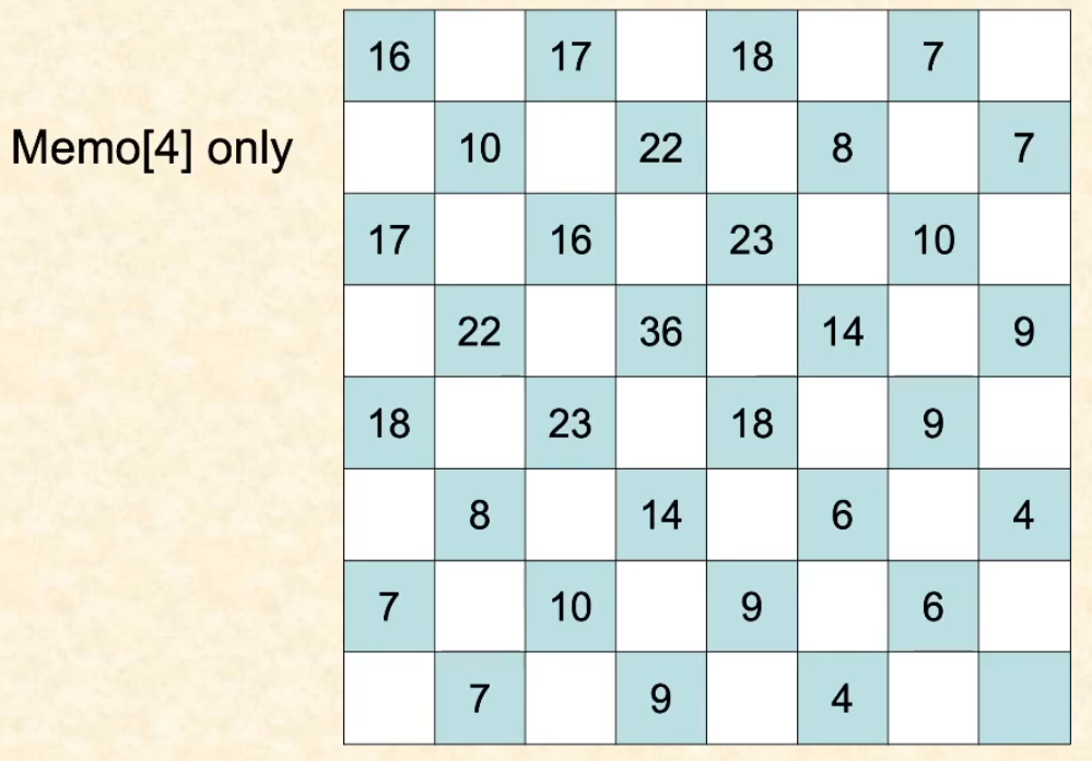
Solve TSP with DP
TSP 问题:给定 n 个城市及它们之间的距离矩阵 dist,找到一条从城市 0 开始,访问所有城市最后回到城市 0 (hamilton cycle)的最短路径。
// TSP 动态规划解法
int tsp(int n, const vector<vector<int>>& cost) {
    // dp[mask][i] 表示从起点 0 出发,经过 mask 表示的所有城市,最后停留在城市 i 的最短路径长度
    vector<vector<int>> dp(1 << n, vector<int>(n, INT_MAX));

    // 初始状态,从起点 0 出发,路径长度为 0
    dp[1][0] = 0;

    // 遍历所有状态 mask
    for (int mask = 1; mask < (1 << n); ++mask) {
        for (int i = 0; i < n; ++i) {
            // 如果城市 i 不在当前 mask 中,跳过
            if (!(mask & (1 << i))) continue;

            // 尝试从集合 mask 中的其他城市转移到 i
            for (int j = 0; j < n; ++j) {
                if (j != i && (mask & (1 << j)) && dp[mask ^ (1 << i)][j] != INT_MAX) {
                    dp[mask][i] = min(dp[mask][i], dp[mask ^ (1 << i)][j] + cost[j][i]);
                }
            }
        }
    }

    // 最后计算从每个终点返回起点的最短路径
    int result = INT_MAX;
    for (int i = 1; i < n; ++i) {
        if (dp[(1 << n) - 1][i] != INT_MAX) {
            result = min(result, dp[(1 << n) - 1][i] + cost[i][0]);
        }
    }

    return result;
}
Difference between DP and Divide-and-Conquer
Divide-and-Conquer 即把一个问题分成 non-overlapping 的子问题,通过一个递推式表示 recursion 关系。我们希望最好能把一个问题切分成 equal size 且参数呈倍数关系的子问题,这样我们更加可能用 master theorem 找出复杂度
比如 $$ 这种递推式.
Divide and Conquer 也分为 Top down 和 Bottom up(combine and conquer)
-
通常 Divide and Conquer:Binary search,quicksort...
-
Combine and Conquer:merge sort...
// Divide and Conquer(top down)
quicksort(array)
	partition;
	quicksort(left)
	quicksort(right)

// Combine and Conquer(bottom up)
mergesort(array)
	merge_sort(left);
	merge_sort(right);
	merge(left, right);
(merge sort 先解决子问题,再 combine 子问题的 solutions;quick sort 先切分成两部分,两部分子问题都解决之后原问题自然解决)
DP 和 Divide-and-Conquer 的区别在于:
DP 使用几个可能 overlapping 的 subproblems 的答案来解决大问题,并通过表格储存先前的 subproblems 答案;
Divide and Conquer 不允许 overlapping subproblems,而是把问题分成几个不相关的子问题,逐个解决。
Lec 24 (Knapsack and Floyd's algorithm)
0-1 knapsack
// 0-1 Knapsack Function
int knapsack(const vector<int>& weights, const vector<int>& values, int W) {
    int n = weights.size();
    vector<vector<int>> dp(n + 1, vector<int>(W + 1, 0));

    for (int i = 1; i <= n; ++i) {
        for (int w = 0; w <= W; ++w) {
            if (weights[i - 1] <= w) {
                dp[i][w] = max(dp[i - 1][w], dp[i - 1][w - weights[i - 1]] + values[i - 1]);
            } else {
                dp[i][w] = dp[i - 1][w];
            }
        }
    }

    return dp[n][W];
}

int main() {
    // Input: weights, values, and max capacity of knapsack
    vector<int> weights = {2, 3, 4, 5};
    vector<int> values = {3, 4, 5, 6};
    int W = 8;

    int max_value = knapsack(weights, values, W);
    cout << "Maximum value that can be obtained: " << max_value << endl;

    return 0;
}
//Maximum value that can be obtained: 10
Floyd's algorithm
const int INF = INT_MAX;

void floydWarshall(vector<vector<int>>& graph) {
    int V = graph.size();
    vector<vector<int>> dist = graph;

    // 三重循环
    for (int k = 0; k < V; ++k) {
        for (int i = 0; i < V; ++i) {
            for (int j = 0; j < V; ++j) {
                // 如果通过 k 能连接 i 和 j,并且减少路径距离
                if (dist[i][k] != INF && dist[k][j] != INF &&
                    dist[i][j] > dist[i][k] + dist[k][j]) {
                    dist[i][j] = dist[i][k] + dist[k][j];
                }
            }
        }
    }

    // 输出结果
    cout << "Shortest distances between every pair of vertices:\n";
    for (int i = 0; i < V; ++i) {
        for (int j = 0; j < V; ++j) {
            if (dist[i][j] == INF) {
                cout << "INF ";
            } else {
                cout << dist[i][j] << " ";
            }
        }
        cout << endl;
    }
}

int main() {
    // 输入:邻接矩阵表示的图 (无穷大用 INF 表示)
    vector<vector<int>> graph = {
        {0, 3, INF, 7},
        {8, 0, 2, INF},
        {5, INF, 0, 1},
        {2, INF, INF, 0}
    };

    floydWarshall(graph);

    return 0;
}

/*
Shortest distances between every pair of vertices:
0 3 5 6
5 0 2 3
3 6 0 1
2 5 7 0
*/
Lab 10 (DP)
Algorithm Problem: Discount DP
given a sequence of orders,for each one, either:
- 25% discount (always have)
- 先前 pay full 五次, 得到一次免费(上限为 5,积累超过 5 次则再多次数不算
要求:minimize cost
Idea: 建立 memo[6][num_orders]
每个 entry 表示
状态转移方程:
for k = 1~5:
第 n 个 order 结束攒了 k 个 fullpay 点数的情况的最优解 =
Min(第 n-1 个 order 结束攒了 k-1 个 fullpay 点数时的钱 + 第 n 个 order pay full 的钱攒点数,
第 n-1 个 order 结束攒了 k 个 fullpay 点数时的钱 + 第 n 个 order 使用 discount 的钱)
for k = 0:
第 n 个 order 结束攒了 k 个 fullpay 点数的情况的最优解 =
Min(
第 n-1 个 order 结束攒了 0 个 fullpay 点数的钱 + 第 n 个 order 使用 discount 的钱,
第 n-1 个 order 结束攒了 5 个 fullpay 点数的钱 + 第 n 个 order 消耗 5 fullpay 免费
)
// How much you pay for a discounted (25% off) meal.
cost discounted(cost full_price) {
    return full_price * 3 / 4;
}

cost best_price(const std::vector<cost>& prices) {
    // NOTE: if you use a bottom-up approach, initialize your table with
    // std::numeric_limits<cost>::max()/4 ... you MUST divide by 4!
    if (prices.size() == 0) {
        return 0;
    }

    std::vector<std::vector<cost>> dp(6, std::vector<cost>(prices.size(), std::numeric_limits<cost>::max()/4));

    // base case: 第一次没有 punch card
    dp[0][0] = discounted(prices[0]);
    dp[1][0] = prices[0];

    for (size_t j = 1; j < prices.size(); ++j) {
        for (size_t i = 0; i < 6; ++i) {
            if (i == 0) {
                // Min(第 j-1 个 order 结束攒了 0 个 fullpay 点数的钱 + 第 j 个 order 使用 discount 的钱,
                //     第 j-1 个 order 结束攒了 5 个 fullpay 点数的钱 + 第 j 个 order 消耗 5 fullpay 免费)
                dp[i][j] = std::min(discounted(prices[j]) + dp[0][j-1], dp[5][j-1]);
            } else {
                // Min(第 j-1 个 order 结束攒了 i-1 个 fullpay 点数时的钱 + 第 j 个 order pay full 的钱攒点数,
                //     第 j-1 个 order 结束攒了 i 个 fullpay 点数时的钱   + 第 j 个 order 使用 discount 的钱)
                dp[i][j] = std::min(prices[j] + dp[i-1][j-1], discounted(prices[j]) + dp[i][j-1]);
            }
        }
    }
    return dp[0][prices.size() - 1];
}