feature map
我们知道对于 x∈Rn linear model h(x,w)=w⊤x can only produce 一个 hyperplane in it. 因而 not very flexible & powerful.
为此我们的解决方法是使用 feature map, 把 x maps to 更加高维度的 (nonlinear) feature space 上, 然后进行学习:

更加直观的是: 当 data live on 一些 nonlinear manifold 上时:
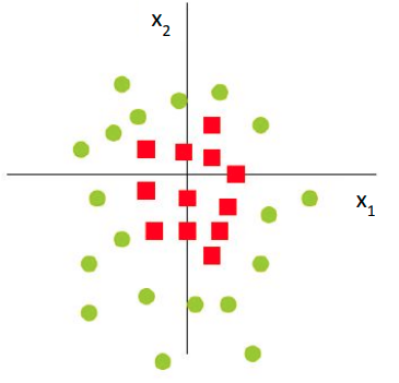
此时 data 是 not linearly separable 的, 因而我们可以把 L2 distance to origin 作为一个 third feature 来进行学习, 即:
$ϕ:(x1,x2)↦(x1,x2,d(x1,x2))或者我们可以直接降低维度,只取这个feature:ϕ:(x1,x2)↦d(x1,x2)$
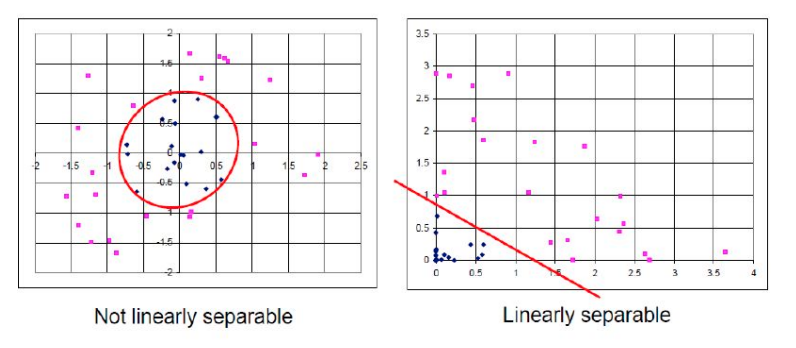
会达到比较好的 regression/classification 效果.
example of solving regression with nonlinear features
for example: ridge regression
linear regression model with feature map:
$h(x,w)=w⊤ϕ(x)=∑j=0Mwjϕj(x)$
object: Least-squares with L2 regression
$J(w)=21∑n=0N(w⊤ϕ(x(n))−y(n))2+2λw⊤w$
Closed form solution:
$w=(Φ⊤Φ+λI)−1y$
这一切都没什么问题但是:
Φ 是一个 N×M 的 matrix
- N : the number of examples
- M : the number of features
因而, 为了计算这个 closed form sol, 我们需要 invert Φ⊤Φ 这个大小是 M×M 的 matrix.
Computational complexity scales with O(M3)
试想: 如果 M 非常大 (远大于 N) 怎么办?
kernel function
define kernel function from feature map
我们定义 kernel function: k:Rn×Rn→R by:
$k(x,x′)=ϕ(x)⊤ϕ(x′)$
两个点的 features 的内积, 即: 这两个点映射到在 feature space 中的 similarity.
for example:
define 一个 kernel function, 反过来看它对应 feature map
因为我们并不是从 w 反推 a ,而是主动把 w 表示成 Φa 的形式。
这种方式等价于在函数空间中搜索解,而不是直接在参数空间中优化。也就是说,即使 Φ 不是满秩的,甚至不是方阵,我们仍然可以这么写。
这实际上是核方法中「代表定理(Representer Theorem)」的体现:最优解 w 总可以表示成样本映射的线性组合,即 w=∑i=1Naiϕ(x(i)) 。